|
Scientific Paper / Artículo Científico |
|
|
|
|
https://doi.org/10.17163/ings.n35.2026.08 |
|
|
|
pISSN: 1390-650X / eISSN: 1390-860X |
|
|
U-NET–BASED SEMANTIC SEGMENTATION OF DEFECTS IN PHOTOVOLTAIC PANELS |
||
|
APLICACIÓN DE MODELOS U-NET PARA SEGMENTACIÓN SEMÁNTICA DE DEFECTOS EN PANELES FOTOVOLTAICOS |
||
|
Franklin
Gómez-López1 |
|
Received: 16-06-2025, Received after review: 18-11-2025, Accepted: 04-12-2025, Published: 01-01-2026 |
|
Abstract |
Resumen |
|
This article presents a study on the semantic segmentation of defects in crystalline-silicon photovoltaic cells using U-Net–based models trained on electroluminescence (EL) images. The dataset combines laboratory-acquired images with a publicly available benchmark, both manually annotated to identify cracks, dark zones, and collector-bar discontinuities. Eight model variants were trained with controlled variations in input resolution, encoder depth, and regularization strategies. Performance was assessed using per-class precision, recall, and F1-score, complemented by visual inspection through heatmaps and overlays and by expert validation. Segmentation was robust for defects with well-defined morphology, such as dark zones and busbars; however, cracks remained more difficult to detect due to their sparse pixel representation and irregular geometry. Alternative architectures (U-Net++ and MAU-Net) were also evaluated but did not yield meaningful improvements over the optimized U-Net configuration. Overall, the results support the use of this approach for automated inspection under controlled conditions, while highlighting the need for future adaptation to more diverse operational scenarios. |
Este artículo presenta un estudio sobre la segmentación semántica de defectos en celdas fotovoltaicas de silicio cristalino mediante modelos basados en U-Net, entrenados con imágenes de electroluminiscencia (EL). Se empleó un conjunto de datos compuesto por imágenes adquiridas en laboratorio y un prototipo público de pruebas, ambos con anotaciones manuales de grietas, zonas oscuras y discontinuidades en barras colectoras. Se entrenaron ocho versiones del modelo, incorporando variaciones controladas en la resolución, la profundidad del codificador y las estrategias de regularización. La evaluación incluyó métricas clase a clase (precisión, recall y F1-score), análisis visual mediante mapas de calor y superposiciones, así como validación por expertos. Si bien la segmentación fue consistente en defectos de morfología clara, como zonas oscuras y barras colectoras, las grietas presentaron mayores dificultades debido a su baja densidad de píxeles y geometría irregular. Asimismo, se analizaron arquitecturas alternativas (U-Net++ y MAU-Net), sin evidenciar mejoras relevantes frente a la configuración optimizada de U-Net. Los resultados respaldan el uso de este enfoque en tareas de inspección automatizada bajo condiciones controladas, y se proponen extensiones para su aplicación en contextos operativos más diversos.
|
|
Keywords: Electroluminescence, predictive maintenance, photovoltaic panels, semantic segmentation, U-Net |
Palabras clave: electroluminiscencia, mantenimiento predictivo, paneles solares, segmentación semántica, U-Net |
|
1,*Faculty of Engineering, Universidad de
Cuenca, Ecuador. 2Department of Electrical, Electronics and
Telecommunications Engineering, Universidad de Cuenca, Ecuador. Corresponding author ✉: danny.ochoac@ucuenca.edu.ec.
Suggested citation: F. Gómez-López, D. Ochoa-Correa and I. Cabrera-Carrera, “U-Net–based semantic segmentation of defects in photovoltaic panels,” Ingenius, Revista de Ciencia y Tecnología, N.◦ 35, pp. 103-113, 2026, doi: https://doi.org/10.17163/ings.n35.2026.08. |
|
1. Introduction
Photovoltaic (PV) energy systems have become a cornerstone of global energy-transition efforts, particularly through distributed generation and decentralized electrification. As PV installations continue to expand, maintaining their operational integrity through accurate diagnostic methods is increasingly critical. Electroluminescence (EL) imaging is widely used to detect structural anomalies in PV modules, including microcracks, broken fingers, and electrically inactive areas [1,2]. Although these defects are often imperceptible during visual inspections, they can progressively degrade module performance over time. Compared with infrared thermography and ultraviolet fluorescence, EL imaging offers superior spatial resolution for detecting early-stage defects without relying on solar irradiance or temperature gradients [3,4]. However, raw EL images often exhibit noise and uneven illumination, which complicate the identification of subtle defect patterns. These limitations underscore the need for advanced image-analysis techniques capable of reliably isolating fine, heterogeneous fault characteristics. Semantic segmentation, which classifies individual pixels into predefined categories, enables precise defect localization in EL images [5, 6]. Among deep learning approaches, convolutional neural networks (CNNs) have demonstrated strong performance in segmentation tasks. In particular, the U-Net architecture is widely adopted for defect detection in PV modules [7]. Originally developed for biomedical image analysis, UNet effectively integrates multi-scale feature extraction with the preservation of spatial resolution, thereby supporting the detection of narrow, localized structures such as microcracks and soldering inconsistencies in photovoltaic cells [8, 9]. Recent research has adapted and refined U-Net variants for PV defect segmentation by incorporating attention mechanisms, residual connections, and hybrid loss functions [10, 11]. These modifications enhance model robustness under varying illumination conditions and improve segmentation accuracy given inter-cell variability in PV module datasets. In addition, publicly accessible EL image datasets, including those released by Fraunhofer ISE and Sandia National Laboratories, support benchmarking and the reproducibility of segmentation results [12, 13]. In this study, multiple U-Net architectures trained on EL images of crystalline-silicon solar cells are implemented and evaluated. Using both proprietary and public datasets, segmentation accuracy across distinct |
defect types is analyzed. The evaluation incorporates parameter-optimization strategies and quantitative comparisons to assess the suitability of U-Net–based methods for supporting automated inspection under controlled laboratory conditions.
2. Materials and Methods
2.1.Datasets
2.1.1. In-house electroluminescence dataset
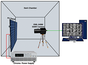
The primary dataset was collected at the Microgrid Laboratory of the University of Cuenca. It comprises 180 solar cells extracted from decommissioned monocrystalline and polycrystalline PV modules. Each cell was imaged under controlled conditions using an OWL 640 M SWIR camera (Raptor Photonics) equipped with an InGaAs sensor sensitive to the 900–1700 nm spectral range. This interval provides improved contrast for defect identification in crystalline silicon compared with sensors operating in the visible spectrum. To ensure uniform illumination, the cells were polarized
using a Chroma DC programmable power supply. The applied current was varied
between To validate the quality of the acquisition system, the Signal-to-Noise Ratio (SNR) was quantified in accordance with the IEC TS 60904-13 standard [14], and defined as equation (1):
Where I1 and I2 are consecutive EL captures and IBG represents the background noise. The experimental setup achieved SNRIEC > 45, meeting the criteria for laboratory measurements. Subsequently, raw EL images underwent preprocessing that included background subtraction, perspective correction, and local contrast enhancement using Contrast Limited Adaptive Histogram Equalization (CLAHE), configured with a clip limit of 2.0 and a tile grid size of 8 × 8. This preprocessing pipeline further improved image quality for segmentation tasks. |
|
2.1.2. Public benchmark dataset
In addition to the proprietary dataset, the publicly available ELPV dataset from the ZAE Bayern group was used for validation. This dataset comprises EL images and corresponding binary crack masks for 2,624 solar cells obtained under factory conditions. Despite differences in resolution and mask structure compared to the in-house dataset, scripts were employed to unify image dimensions and encoding formats. By integrating both internal and external datasets, the combined dataset supports model generalization across different panel types and acquisition configurations. Previous studies adopting similar hybrid-dataset strategies have reported improved segmentation accuracy and cross-domain robustness.
2.1.3. Data Integration and Preprocessing
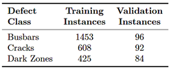
Since the public ELPV dataset provided only binary crack masks, a re-annotation process was conducted using the Supervisely platform [15], to manually generate ground-truth masks for the missing classes. This ensured that the in-house and public datasets shared a consistent multi-class annotation schema (background and three defect classes). Table 1 summarizes the distribution of defect instances across the training and validation sets. The dominance of the busbar class is expected, as this structural component is present in every cell. This class imbalance was addressed during training through the data-augmentation pipeline described in the following section.
Table 1. Distribution of defect instances in the Training and Validation sets
2.2.Acquisition Setup and Pipeline
The complete acquisition setup is depicted in Figure 1. The SWIR camera was positioned orthogonally above the cell, maintaining a fixed lens-to-target distance of 50 cm. Imaging was performed in a darkened chamber to eliminate ambient-light interference. Nonuniformity correction (NUC) was applied using a threepoint method (Offset + Gain + Dark) to minimize fixed-pattern noise. |
Figure 1. Experimental setup showing the OWL 640 M SWIR camera and the PV module under test.
All image-processing steps were implemented in Python using the OpenCV and NumPy libraries. Evaluation metrics, including the Contrast Improvement Ratio (CIR), Peak-to-Low ratio (PL), and visual heatmaps, were extracted from each preprocessed image.
2.3.Annotation Consistency
Inter-annotator agreement was periodically assessed using the Dice coefficient, see equation (2):
Where A and B represent pixel sets annotated independently by different evaluators. A mean Dice score above 0.85 was consistently maintained throughout the annotation process. These datasets served as the basis for training and validating the segmentation models described in the following section.
2.4. Model Architecture
2.4.1. Standard U-Net with VGG16 encoder
The architecture employed in this study is based on UNet, originally developed for biomedical image segmentation [7]. Its encoder-decoder structure enables pixellevel classification by integrating multi-scale features while preserving spatial resolution. In this implementation, the contracting path is replaced with a VGG16 encoder pre-trained on the ImageNet dataset [16].
|
|
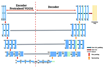
Since the standard VGG16 architecture expects a three-channel input (RGB) and EL images are singlechannel (grayscale), the input was adapted during preprocessing by replicating the single channel three times to match the expected tensor dimensions without modifying the pre-trained weights. This configuration enhances feature representation at the input stage and improves convergence stability [17]. Each downsampling stage in the encoder includes two 3×3, convolutional layers followed by a 2×2 maxpooling operation. The encoder generates five feature maps of increasing depth. To expand the receptive field while preserving spatial dimensions, the bottleneck kemploys dilated convolutions with a fixed dilation rate of r = 2. Figure 2 illustrates the U-Net variant adopted in this study, which incorporates dilated convolutions in the bottleneck to expand the receptive field without increasing the number of parameters [8, 18].
Figure 2. U-Net architecture with VGG16 encoder and dilated convolution bottleneck.
2.4.2. Layer configuration, activation functions and multi-class output
All convolutional layers use ReLU activation functions and batch normalization to improve training stability. A dropout rate of 0.2 is applied in the bottleneck and decoder layers to mitigate overfitting. The decoder upsamples feature maps using transposed convolutions, with skip connections linking each upsampling block to the corresponding encoder stage. The output layer consists of a 1×1 convolution followed by a softmax activation to produce a pixel-wise probability distribution over C defect classes, see equation (3):
Where zi,j,c is the raw score for class c at pixel (i, j), and C = 3 represents the defect classes: cracks, dark zones, and busbars. |
Input images are grayscale EL images resized to 256×256 pixels. Output segmentation masks preserve the same resolution. The entire pipeline was implemented using the PyTorch framework. Prior studies indicate that the combination of skip connections, a symmetric architecture, and multi-class outputs is well-suited to detecting subtle defect patterns in EL images [10, 19]. Alternative architectures, such as MAU-Net with spatial-channel attention mechanisms, were also examined for comparison and are discussed in the Results and Discussion.
2.5.Training Process
2.5.1. Preprocessing and data augmentation
Before training, all EL images were resized to a standard resolution of 256 × 256 pixels. To distinguish image features from categorical labels effectively during resizing, bilinear interpolation was applied to the grayscale EL images, whereas nearest-neighbor interpolation was used for the masks to preserve discrete class values. The pixel values were then normalized to the [0, 1] range to ensure a consistent input format and enhance model stability. Each grayscale input image was paired with a one-hot encoded mask representing the three defect categories: cracks, dark zones, and busbars. To expand the variability of training samples, data augmentation was performed on-the-fly. Transformations included horizontal and vertical flipping, random rotations up to ±15◦, zoom scaling between 0.9× and 1.1×, and elastic deformations. These augmentations were applied probabilistically using the Albumentations library, ensuring that the structural integrity of the masks was maintained. This augmentation approach enhances generalization, particularly for models trained on small or homogeneous EL datasets. Similar strategies have been used to address class imbalance and improve sensitivity to rare defect patterns.
2.5.2. Configuración de hiperparámetros y programador de tasa de aprendizaje
Model training was conducted using the Adam optimizer, which combines adaptive gradient estimation with momentum. The selected hyperparameters were as follows:
· Learning rate: lr = 0.0018 · First moment decay rate: β1 = 0.9 · Second moment decay rate: β2 = 0.999 · Numerical stability term: ϵ = 1 × 10⁻⁸ |
|
Training was driven by the standard Categorical Cross-Entropy loss function, see equation (4):
Where yi,c is the true label (one-hot
encoded) and A step-based learning-rate scheduler was used to improve convergence and avoid local minima. The learning rate was reduced by a factor γ = 0.05 every 8 epochs. This gradual decay facilitated fine-tuning during later training phases. Early stopping was enabled to terminate training if the validation loss did not improve for 10 consecutive epochs. |
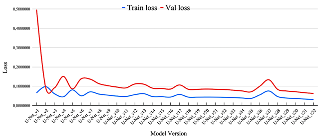
The training process was iterative. Each subsequent model version was initialized with the weights from the best-performing previous version, allowing progressive refinement without reinitialization. The final model version (U-Net_v32) was trained for 48 epochs, with the lowest validation loss observed at epoch 26. The corresponding values for training and validation loss are shown in equation (5):
Figure 3 displays the evolution of loss values across model versions. These visualizations aided in monitoring training behavior and validating incremental improvements.
|
|
Figure 3. Evolution of training and validation loss values across iterative U-Net model versions. |
|
To ensure reproducibility, all experiments were conducted using the PyTorch framework (v2.3.1) in Google Colab Pro environment equipped with an NVIDIA T4 GPU. A fixed random seed of 42 was set for weight initialization and data partitioning. Training was performed with a batch size of 16 for 48 epochs, using the Adam optimizer with an initial learning rate of 0.0018 and a step-based decay scheduler (step_size = 8, γ = 0.05). The best model weights were saved based on the minimum validation loss, which typically converged around epoch 26. The final U-Net model has a storage footprint of approximately 233 MB. During the inference phase, processing a batch of 16 images (256×256 pixels) took an |
average of 0.52 seconds, translating to an inference latency of approximately 32.6 ms per image (∼30 FPS).
2.6.Evaluation Metrics
2.6.1. Precision, Recall and F1-score
To assess model performance at the pixel level, three complementary metrics were computed: precision, recall, and F1-score. These metrics were calculated independently for each defect class — cracks, dark zones, and busbars — as recommended in segmentation studies focused on PV defect detection [8, 18]. |
|
Precision quantifies the proportion of correctly identified defect pixels among all pixels predicted as defective, see equation (6):
Where TP represents true positives (correctly predicted defect pixels) and FP denotes false positives (non-defect pixels incorrectly predicted as defects). Recall, also referred to as sensitivity, measures the proportion of actual defect pixels that are correctly identified, see equation (7):
With FN indicating false negatives (defect pixels that the model failed to detect). The F1-score, calculated as the harmonic mean of precision and recall, provides a balanced metric for evaluating classification accuracy, see equation (8):
These metrics are particularly relevant in multiclass segmentation tasks involving class imbalance and subtle morphological features, such as microcracks [10].
2.6.2. Validation Strategy and Confusion Matrix
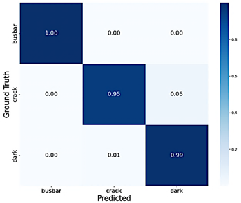
To evaluate model performance and monitor convergence during the iterative training of 32 model versions, a fixed hold-out validation strategy was employed instead of k-fold cross-validation. The dataset was strictly partitioned into three independent subsets: training (1453 images, including augmented data), validation (96 original images), and testing. This approach ensured that the evaluation metrics remained comparable across different training epochs and hyperparameter adjustments, while avoiding data leakage from the augmentation process. A confusion matrix was generated using the best performing model (U-Net_v32) on the validation set to visualize class-specific prediction errors. Figure 4 presents the normalized confusion matrix. A higher misclassification rate was observed for the crack class, which is attributed to the sparse and fragmented spatial distribution of this defect type compared with the more distinct features of busbars and dark zones. |
Figure 4. Normalized confusion matrix for U-Net_v32 evaluated on validation data.
This validation protocol enables a clear assessment of the model’s generalization capability on unseen data, with particular emphasis on the correct identification of minority defect classes.
3. Results and Discussion
3.1.Performance by Defect Class
3.1.1. Segmentation of cracks, dark zones and busbars
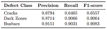
The segmentation performance of the trained U-Net models varied across defect classes. As shown in Table 2, the highest F1-score was obtained for dark zones, which typically occupy larger, more homogeneous regions. Busbar discontinuities also exhibited consistent segmentation performance, particularly when there was clear contrast against the cell background.
Table 2. Mean segmentation metrics by class (UNet_v32).
Cracks, in contrast, posed greater challenges. These defects are narrow, irregular, and frequently overlap with low-contrast textures. Consistent with prior studies by Pratt et al. [8] and Deitsch et al. [18], the crack class exhibited lower precision and recall, attributable to its pixel-level sparsity and morphological variability. |
|
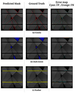
Qualitative inspection further indicated that cracks located near the cell edges or partially occluded by finger metallization were more frequently missed. These observations are consistent with benchmarking results obtained from EL datasets such as ELPV [19]. Figure 5 illustrates representative segmentation outcomes and their comparison with the ground truth for the three defect types.
Figure 5. Examples of predicted segmentation masks for (a) cracks, (b) dark zones, and (c) busbars. Each row shows the original EL image, the predicted segmentation overlaid on the image, the ground truth mask overlaid, and an error map in which cyan represents false positives (FP) and orange represents false negatives (FN).
For each class, the figure shows the original EL image, the predicted mask overlaid on the image, the corresponding ground truth mask, and an error map highlighting discrepancies. In the error maps, cyan denotes false positives (pixels incorrectly predicted as defective), whereas orange denotes false negatives (defect pixels not detected by the model). For cracks, the error maps reveal fragmented boundaries, particularly in regions with weak luminescence, which corroborates the limitations observed in the quantitative evaluation. For dark zones and busbars, the false-positive and false-negative regions are minimal, consistent with their comparatively higher F1- scores.
3.1.2. Error analysis and class imbalance
A persistent challenge during training was class imbalance. Background pixels accounted for over 85% of the dataset, while cracks represented less than 5%. This imbalance affected both the optimization process and |
metric interpretation, as the loss function tended to prioritize the majority classes. To mitigate this issue, class-weighted loss functions were employed, assigning higher penalties to errors in underrepresented classes. In addition, data augmentation was specifically targeted to increase the number of samples containing cracks. These adjustments improved the model’s sensitivity to minority classes without compromising training stability. As illustrated in the normalized confusion matrix in Figure 4, the highest misclassification rates occurred for the crack class, particularly in cases where diffuse or low-contrast defects were mistaken for dark zones. False positives in the busbar class occasionally appeared near cell edges. These errors were attributed to abrupt brightness variations caused by non-uniform illumination or optical reflections during image acquisition.
3.2.Comparative Analysis Between Model Version
3.2.1. Iterative evaluation from U-Net_v24 to U-Net_v322
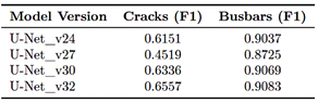
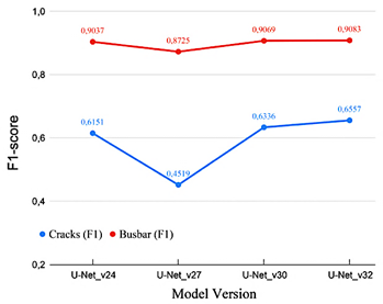
An iterative evaluation process was conducted across model versions from U-Net_v24 to U-Net_v32. Each iteration introduced controlled modifications aimed at improving performance under constrained data and hardware conditions. These adjustments included increasing input resolution from 128 × 128 to 256 × 256 pixels, varying dropout rates between 0.15 and 0.3, and reducing batch size to accommodate higher-resolution inputs within the available GPU memory. Table 3 summarizes the evolution of F1-scores for the crack and busbar classes.
Table 3. F1-score evolution for crack and busbar segmentation
Improvements were most evident in the crack class, where earlier model versions failed to detect faint linear patterns, particularly near cell boundaries. The use of higher input resolution and deeper encoder configurations in U-Net_v30 and U-Net_v32 improved the network’s ability to preserve detailed features during the downsampling process. Figure 6 illustrates the progression of F1-scores across model versions. |
|
Figure 6. F1-score progression across model versions (Cracks and Busbars).
These outcomes are consistent with previous observations indicating that gradual refinement of hyperparameters and input structure, rather than radical architectural changes, tends to yield more reliable improvements in segmentation models trained on limited or domain-specific datasets.
3.2.2. Discussion on alternative architectures: U-Net++, MAU-Net
Two U-Net variants, U-Net++ and MAU-Net, were evaluated under the same training conditions. UNet++ adds nested skip connections to enhance gradient flow and semantic fusion, while MAU-Net introduces spatial and channel attention to prioritize relevant features and suppress noise. Both variants slightly improved recall for cracks in low-contrast regions; however, the overall F1-score gain was marginal (below 1.5%) compared to U-Net_v32. MAU-Net also incurred a 35% increase in inference time. Given these trade-offs, the baseline U-Net was preferred because it offers greater stability, lower complexity, and more consistent performance across defect types.
3.3.Visual and Qualitative Validation
3.3.1. Heatmaps and overlays on individual cells
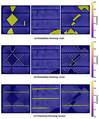
In addition to quantitative metrics, visual inspection is essential for understanding model behavior under realistic diagnostic conditions. To support this, heatmaps were generated from softmax output probabilities for each defect class and overlaid on the original electroluminescence (EL) images to visualize the model’s prediction confidence.
|
As illustrated in Figure 7, dark zones were consistently identified due to their well-defined boundaries and contrast characteristics. In comparison, crack predictions occasionally missed fragmented sections near cell borders or beneath finger metallization, where luminescence levels were lower. These observations are consistent with findings reported in prior evaluations using EL datasets such as ELPV [19] and with approaches that employ visual overlays for segmentation verification [8].
Figure 7. Overlay examples: (a) dark zones correctly predicted; (b) partial crack detection; (c) overprediction in the busbar area.
3.3.2. Expert evaluation and prediction visualization
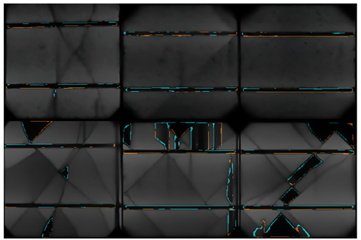
To complement automated performance metrics, a qualitative review was conducted by three experts in PV diagnostics. Each expert independently evaluated a set of 30 predicted segmentation masks, focusing on contour accuracy, spatial consistency, and interpretability. The assessment criteria were aligned with visual inspection standards adapted from IEC TS 60904-13 for EL image analysis [14]. Most predictions for dark zones and busbars were considered highly consistent with diagnostic expectations, with minimal segmentation discrepancies. Figure 8 presents representative error maps for these classes. Cyan pixels indicate false positives, and orange pixels represent false negatives. In most cases, only minor misalignments were observed, often appearing as thin traces resulting from slight differences in edge thickness between the predicted masks and the ground truth annotations. |
|
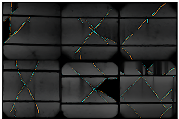
Crack segmentation was more challenging. Some prediction masks exhibited irregular contours or overestimated defect regions in low-contrast areas. Figure 9 provides examples of these error cases. Prominent orange traces denote missed crack segments (false negatives), while cyan regions correspond to false-positive predictions in ambiguous zones. These patterns frequently coincided with electroluminescence gradients induced by inconsistent polarization currents or subtle misalignment during image acquisition. This qualitative analysis revealed patterns that are useful for guiding model refinement. Future implementations may benefit from selective post-processing or attention-based modules aimed at reducing false positives and improving spatial resolution in regions where defect boundaries are poorly defined. Overall, the combination of visual overlays, probability-based heatmaps, and expert assessment offered a multidimensional perspective on model performance that complemented standard metrics such as F1-score and confusion matrices.
Figure 8. Representative error maps for correctly segmented dark zones and busbars. Cyan indicates false positives, and orange denotes false negatives.
Figure 9. Examples of segmentation errors. Missed cracks are highlighted in orange, while false positives in lowcontrast areas are shown in cyan. |
4. Conclusions
This study examined U-Net-based convolutional architectures for semantic segmentation of defects in crystalline silicon photovoltaic cells using EL imaging. A dual-source dataset, including in-house and public EL images, was used for training and evaluation, with manual annotations for cracks, dark zones, and busbar discontinuities. The models performed consistently on defects with clear morphology and strong contrast, such as dark zones and interrupted busbars. Cracks remained the most difficult class to segment, due to their sparse distribution and irregular geometry, consistent with previous findings [8, 18]. From a practical perspective, the present results are constrained by several factors. Many cracks appear as thin, irregular trajectories with very low pixel density and subtle contrast relative to the surrounding material, which leads the network to miss very short or faint segments and, in some cases, to confuse small crack fragments with background texture or acquisition artefacts. In addition, the mandatory resizing of single-cell EL images to 256 × 256 pixels, required by the VGG16-based encoder, may compress the thinnest structures into only a few pixels and thus limit sensitivity to the smallest defects. The dataset size and diversity are also limited, since all images were captured under controlled laboratory conditions and do not include field EL acquisitions with varying bias currents, surface contamination, or optical non-uniformities. These factors should be considered when extrapolating the reported performance to other setups or operating conditions. Eight model versions were evaluated using a structured training workflow with progressive modifications in encoder depth, input resolution, regularization, and learning strategies. The final configuration (U-Net_v32) provided the best balance between accuracy and computational efficiency. Variants such as U-Net++ and MAU-Net yielded only minor performance gains at the cost of increased inference time [11]. Quantitative metrics, visual outputs, and expert assessments were jointly used to evaluate model behavior. This integrated validation confirmed the utility of U-Net models for defect localization under controlled conditions. Future work should focus on (1) expanding the dataset with field-acquired EL images that capture real-world variability, and (2) developing and integrating post-processing techniques to reduce false positives and improve boundary accuracy in low-contrast regions. These developments would enhance the applicability of segmentation models in operational PV diagnostics and manufacturing quality control. |
|
Acknowledgments
The authors express their appreciation to the Microgrid Laboratory of the University of Cuenca for providing the facilities and technical support necessary for this study. Special thanks are extended to the laboratory staff, Vinicio Iñiguez, Edisson Villa, and Pablo J. Delgado, for their assistance during the experimental phase.
Rol de autores
· Franklin Gómez-López: conceptualization, data curation, formal analysis, investigation, methodology, software, validation, visualization, writing – original draft. · Danny Ochoa-Correa: formal analysis, funding acquisition, investigation, project administration, resources, supervision, writing – review & editing. · Isabel Cabrera-Carrera: data curation, formal analysis, investigation, methodology, supervision, writing – review & editing.
References
[1] K. G. Bedrich, M. Bliss, T. R. Betts, and R. Gottschalg, “Electroluminescence imaging of PV devices: Determining the image quality,” in 2015 IEEE 42nd Photovoltaic Specialist Conference (PVSC). IEEE, Jun. 2015, pp. 1–5. [Online]. Available: https://doi.org/10.1109/PVSC.2015.7356011 [2] T. Fuyuki and A. Kitiyanan, “Photographic diagnosis of crystalline silicon solar cells utilizing electroluminescence,” Applied Physics A, vol. 96, no. 1, pp. 189–196, Dec. 2008. [Online]. Available: http://doi.org/10.1007/s00339-008-4986-0 [3] M. Akram and J. Bai, “Defect detection in photovoltaic modules based on image-to-image generation and deep learning,” Sustainable Energy Technologies and Assessments, vol. 82, p. 104441, Oct. 2025. [Online]. Available: http://doi.org/http://doi.org/ [4] J. Wang, L. Bi, P. Sun, X. Jiao, X. Ma, X. Lei, and Y. Luo, “Deep-learning-based automatic detection of photovoltaic cell defects in electroluminescence images,” Sensors, vol. 23, no. 1, p. 297, Dec. 2022. [Online]. Available: http://doi.org/10.3390/s23010297 |
[5] Q. Liu, M. Liu, C. Wang, and Q. J. Wu, “An efficient CNN-based detector for photovoltaic module cells defect detection in electroluminescence images,” Solar Energy, vol. 267, p. 112245, Jan. 2024. [Online]. Available: http://doi.org/10.1016/j.solener.2023.112245 [6] J. Fioresi, D. J. Colvin, R. Frota, R. Gupta, M. Li, H. P. Seigneur, S. Vyas, S. Oliveira, M. Shah, and K. O. Davis, “Automated defect detection and localization in photovoltaic cells using semantic segmentation of electroluminescence images,” IEEE Journal of Photovoltaics, vol. 12, no. 1, pp. 53–61, Jan. 2022. [Online]. Available: http://doi.org/10.1109/jphotov.2021.3131059 [7] O. Ronneberger, P. Fischer, and T. Brox, U-Net: Convolutional Networks for Biomedical Image Segmentation. Springer International Publishing, 2015, pp. 234–241. [Online]. Available: http://doi.org/10.1007/978-3-319-24574-4_28 [8] L. Pratt, D. Govender, and R. Klein, “Defect detection and quantification in electroluminescence images of solar PV modules using U-net semantic segmentation,” Renewable Energy, vol. 178, pp. 1211–1222, Nov. 2021. [Online]. Available: http://doi.org/10.1016/j.renene.2021.06.086 [9] H. Eesaar, S. Joe, M. U. Rehman, Y. Jang, and K. T. Chong, “SEiPV-net: An efficient deep learning framework for autonomous multi-defect segmentation in electroluminescence images of solar photovoltaic modules,” Energies, vol. 16, no. 23, p. 7726, Nov. 2023. [Online]. Available: https://doi.org/10.3390/en16237726 [10] M. R. U. Rahman and H. Chen, “Defects inspection in polycrystalline solar cells electroluminescence images using deep learning,” IEEE Access, vol. 8, pp. 40 547–40 558, 2020. [Online]. Available: http://doi.org/10.1109/access.2020.2976843 [11] R. A. Mamun Rudro, K. Nur, F. A. Al Sohan, M. Mridha, S. Alfarhood, M. Safran, and K. Kanagarathinam, “SPF-Net: Solar panel fault detection using U-net based deep learning image classification,” Energy Reports, vol. 12, pp. 1580–1594, Dec. 2024. [Online]. Available: http://doi.org/10.1016/j.egyr.2024.07.044 [12] S. Deitsch, V. Christlein, S. Berger, C. Buerhop- Lutz, A. Maier, F. Gallwitz, and C. Riess, “Automatic classification of defective photovoltaic module cells in electroluminescence images,” Solar Energy, vol. 185, pp. 455–468, Jun. 2019. [Online]. Available: http://doi.org/10.1016/j.solener.2019.02.067 |
|
[13] U. Hijjawi, S. Lakshminarayana, T. Xu, and M. Rahman, “A benchmarking study of instance segmentation methods for photovoltaic cell defect detection using electroluminescence images,” Solar Energy, vol. 303, p. 114083, Jan. 2026. [14] IEC, IEC Technical Specification 60904-13. Photovoltaic devices - Part 13: Electroluminescence of photovoltaic modules. InternationalElectrotechnicalCommission, 2018. [Online]. Available: http://doi.org/10.4229/35thEUPVSEC20182018-5CV.3.15 [15] Supervisely. (2023) Supervisely computer vision platform. Supervisely OÜ. [Online]. Available: https://upsalesiana.ec/ing35ar8r2 [16] K. Simonyan and A. Zisserman, “Very deep convolutional networks for large-scale image recognition,” 2014. [17] A. Sohail, N. Ul Islam, A. Ul Haq, S. Ul Islam, I. Shafi, and J. Park, “Fault detection and computation of power in PV cells under faulty conditions using deep-learning,” Energy Reports, vol. 9, pp. 4325–4336, Dec. 2023. |
[18] S. Deitsch, C. Buerhop-Lutz, E. Sovetkin, A. Steland, A. Maier, F. Gallwitz, and C. Riess, “Segmentation of photovoltaic module cells in uncalibrated electroluminescence images,” Machine Vision and Applications, vol. 32, no. 4, May 2021. [19] C. Buerhop-Lutz, S. Deitsch, A. Maier, F. Gallwitz, S. Berger, B. Doll, J. Hauch, C. Camus, and C. Brabec, “A benchmark for visual identification of defective solar cells in electroluminescence imagery,” 35th European Photovoltaic Solar Energy Conference and Exhibition; 1287-1289, 2018. [Online]. Available: http://doi.org/10.4229/35THEUPVSEC20182018-5CV.3.15 |