Scientific Paper / Artículo Científico
		https://doi.org/10.17163/ings.n35.2026.07
		pISSN: 1390-650X / eISSN: 1390-860X
ESTIMATION OF EMISSIONS FROM FAILURES IN OTTO ENGINES USING CONVOLUTIONAL NEURONAL NETWORKS

ESTIMACIÓN DE EMISIONES POR FALLOS EN MOTORES OTTO MEDIANTE REDES NEURONALES CONVOLUCIONALES

Elmer I. Arias-Montaño¹, Rogelio S. León-Japa^1,*,

Pedro García-Jaramillo¹ , José Maldonado-Ortega²

Received: 24-05-2025, Received after review: 05-11-2025, Accepted: 20-11-2025, Published: 01-01-2026

Abstract	Resumen
This study applies a machine learning technique, specifically Convolutional Neural Networks (CNNs), to predict pollutant emissions resulting from failures in actuators and components of Otto engines. The work addresses the current lack of non-intrusive methods that exploit signals already available in the vehicle to estimate, with high accuracy, emissions associated with failures in the injection, ignition, and air intake systems. Concentrations of CO (% carbon monoxide), CO₂ (% carbon dioxide), HC (unburned hydrocarbons, ppm), and O_v (% oxygen) are quantified by analyzing the Manifold Absolute Pressure (MAP) sensor signal under a rigorous sampling and signal processing protocol. Optimal features are extracted from the MAP signal based on their informational relevance and discriminative capacity. These features are obtained through spectrographic transformation, enabling the construction of a robust database. The resulting dataset serves as an effective input for CNN training, achieving emission prediction errors below 1%.	En este estudio se implementa una técnica de aprendizaje automático, concretamente redes neuronales convolucionales (CNN, por sus siglas en inglés), con el objetivo de predecir las emisiones contaminantes producidas por fallos en actuadores y componentes de motores Otto. Así pues, el problema de investigación abordado en este trabajo es la ausencia de métodos no intrusivos que, a partir de señales ya disponibles en el vehículo, permitan estimar con alta precisión las emisiones asociadas a fallas en sistemas de inyección, encendido y admisión de aire. Se cuantifican los niveles de CO (monóxido de carbono, %), CO₂ (dióxido de carbono, %), HC (hidrocarburos no quemados en ppm) y O₂ (oxígeno, %) a partir del análisis de la señal proveniente del sensor MAP (Manifold Absolute Pressure). Para ello, se adopta un protocolo riguroso de muestreo y procesamiento de la señal. La extracción de características óptimas del sensor MAP se basa en su relevancia informativa y capacidad de discriminación, determinadas mediante la transformación espectrográfica de la señal, lo que permite construir una base de datos robusta. Esta base sirve como entrada eficaz para el entrenamiento de la CNN, con la cual se logra un error de predicción inferior al 1 %.
*Keywords:* Convolutional neural networks (CNN), emissions, estimation, Otto engines, machine learning.	*Palabras clave:* CNN, emisiones, estimación, motor Otto, redes neuronales convolucionales, machine learning.

^1,*Grupo de Investigación en Movilidad, Vehículos y Transporte (eX- MoVeT), Carrera de Ingeniería Automotriz, Universidad Nacional de Loja, Loja-Ecuador. Corresponding author ✉: rleonj@outlook.es.

²Grupo de Investigación en Movilidad Inteligente (GMovInt), Carrera de Ingeniería Automotriz, Universidad Politécnica Salesiana, Guayaquil-Ecuador

Suggested citation: E. I. Arias-Montaño, R. S. León-Japa, P. García-Jaramillo and J. Maldonado-Ortega “Estimation of emissions from failures in Otto engines using convolutional neuronal networks,” Ingenius, Revista de Ciencia y Tecnología, N.◦ 35, pp. 90-102, 2026, doi: https://doi.org/10.17163/ings.n35.2026.07.

1. Introduction

Currently, emissions from alternative internal combustion engines (MCIA) are among the most significant sources of atmospheric pollution in urban areas worldwide. These emissions degrade air quality and pose an environmental challenge of increasing concern.

In contrast, in spark-ignition engines (MEP) the air fuel mixture is not always completely burned during the ignition phase due to inefficiencies arising from variations in temperature and load, changes in engine speed (rpm), and fluctuations in internal pressure [1]. Therefore, to evaluate combustion efficiency, it is necessary to quantify the main emitted pollutants, namely carbon monoxide (CO), carbon dioxide (CO₂), unburned hydrocarbons (HC), nitrogen oxides (NO_x), and oxygen (O₂) [2, 3].

Accordingly, it becomes essential to adopt advanced methodologies that integrate computational mathematics with artificial intelligence tools [4, 5]. Such approaches enable more precise detection of faults in the components and actuators of alternative internal combustion engines (MCIA), as well as a more detailed characterization of exhaust gas emissions [6].

Sapio et al. [7] developed a hybrid modeling approach for selective catalytic reduction (SCR) systems. Specifically, they employed recurrent neural networks (RNNs) and subsequently used feedforward neural networks (FFNNs) to predict both the outlet temperature of the catalytic system (SC) and pollutant concentrations, particularly NO_x and NH₃ [8].

The use of advanced supervised learning techniques, including artificial neural networks (ANNs) bidirectional convolutional networks (CNN-BiLSTM), support vector machines (SVMs), and the extreme gradient boosting algorithm (XGBoost), has proven to be an effective alternative for improving odor assessment in vehicle interiors [9].

Cesur and Uysal [10] demonstrated that using methanol–gasoline fuel blends in spark-ignition engines (MEP) increases effective power by 3.7 % while notably reducing NO_x and HC levels. In addition, their model enabled the prediction of engine performance parameters and emissions with accuracies of 99 % and 98 %, respectively.

To estimate CO₂ emissions, studies have employed various algorithms, including linear regression, decision trees, and neural networks. Collectively, their findings confirm the high effectiveness of machine learning approaches for accurate prediction in vehicular emissions [11].

Li et al. [12] developed an improved model for misfire detection in gasoline engines based on YOLOv8,

optimized with BiFormer and CBAM modules to enhance feature extraction from acoustic signals. Engine signals were transformed via wavelet analysis into time–frequency images for network training, achieving an accuracy of 99.71% and thereby outperforming the original YOLOv8 approach [13–15].

The present research focuses on analyzing intake manifold pressure using the signal recorded by the MAP sensor in spark-ignition engines (MEP). The study addresses the need for a rapid, low-cost, and minimally invasive method to diagnose faults in gasoline engines and estimate their exhaust emissions. In contrast, current approaches often rely on complex physical models or test benches, which increase both cost and measurement time [16].

Accordingly, the problem can be summarized as determining how to leverage the information contained in a single MEP sensor to quantitatively estimate multiple exhaust emissions under different incipient fault conditions using deep learning techniques [17, 18]. In this sense, the proposed methodology represents a relevant advancement for both exhaust-emission prediction and fault detection in MEP engines.

The article is organized as follows: Section 2 describes the experimental configuration, the data acquisition procedure, the construction of the spectrograms, and the CNN design. Section 3 presents the emission-prediction results and the comparative statistical analysis. Finally, Section 4 summarizes the main conclusions and outlines future work.

2. Materials and methods

The following section presents the proposed advanced diagnostic approach, along with the implemented experimental configuration and instrumentation, which are minimally invasive in nature. This section also details the sampling conditions, the data acquisition methodology, the processing of the MAP sensor signal, and the procedure for selecting the spectrograms used to train the convolutional neural network (CNN). In addition, it describes the development of the algorithm designed for emission prediction and fault detection in the system.

2.1.Experimental configuration and instrumentation

The proposed approach aims to avoid disassembling vehicle components and systems by enabling fault detection and exhaust-emission prediction through a minimally invasive method. To achieve this objective, samples of the vacuum generated in the spark-ignition

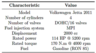
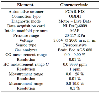
engine (MEP) are acquired using the voltage signal produced by the manifold absolute pressure (MAP) sensor as the information source.

Table 1 summarizes the technical characteristics of the MEP engine used in the study, whereas Table 2 presents the instrumentation employed during the experimental process.

Table 1. Technical characteristics of the MEP engine

Table 2. Instrumentation used in the study

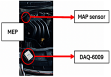
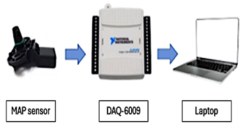
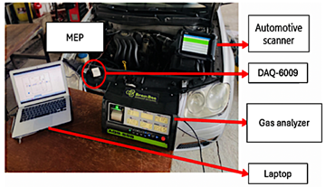
Figure 1 illustrates the main components used in this study, including the manifold absolute pressure (MAP) sensor, the DAQ-6009 data acquisition board, and a laptop computer serving as the processing unit. Figure 2 shows the connection scheme established between the DAQ-6009 board, the MAP sensor, and the experimental unit selected for testing, specifically a 2011 Volkswagen Jetta vehicle.

Figure 1. Instrumentation used in the MEP engine

The MAP sensor is an original vehicle component present in most modern Otto engines, making the proposed approach economical and easily replicable without the need to add external hardware.

Figure 2. Connection scheme for MAP sensor signal acquisition

2.2.Sampling conditions

The MAP sensor installed in the experimental unit was used to capture the voltage signal, due to its strategic location in the intake manifold of the spark-ignition engine (MEP). In parallel, exhaust gas emission samples were collected, including carbon monoxide (CO) and carbon dioxide (CO₂), both expressed percentages, unburned hydrocarbons (HC) expressed in parts per million (ppm), and oxygen (O₂), also expressed as a percentage. These measurements were obtained using a gas analyzer, while the MAP sensor signal was acquired through the DAQ-6009 board using LabVIEW 2024, which enabled real-time monitoring.

During data collection, both the MAP sensor signal and exhaust gas emissions were recorded at a constant engine speed of 2500 rpm under static test conditions in the experimental unit. The MEP operating temperature was maintained between 90 to 98 °C, and an automotive scanner was used to verify and monitor the engine’s key parameters in real time.

According to the pre-experimental study by Contreras et al. [19], the MAP sensor signal exhibits highfrequency peaks. Consequently, the authors recommend acquiring data at a rate of 10 kHz over an interval of 5 s to satisfy the Nyquist criterion.

The absolute pressure in the intake manifold is directly related to engine load, volumetric efficiency, and combustion dynamics. Therefore, its variations contain information about faults in the intake, injection, and ignition systems. Previous studies by this research group have shown that, when properly processed, the MAP signal enables discrimination of operating conditions and certain fault types with good sensitivity [2], [19]. By

relying exclusively on the MAP sensor signal, the proposed approach remains minimally invasive, since exhaust ducts are not manipulated, additional intrusive sensors are not required, and overall system complexity is reduced.

In accordance with this recommendation, the DAQ- 6009 board was configured with a sampling rate of 5 kHz for the samples to read parameter, an acquisition frequency of 10 kHz, and a duration of 5 s for each experimental treatment, using a differential connection mode. The data-collection order was planned in Minitab through a design of experiments (DOE). Accordingly, eight base treatments were defined, and to increase the statistical robustness and representativeness of the dataset, ten replicates were performed for each treatment [1].

2.3.Data collection procedure

Figure 3 presents the main physical components used to diagnose faults in components and actuators and to predict exhaust gas emissions. These elements include an automotive scanner, the DAQ-6009 data acquisition board, a Brain Bee gas analyzer, and a laptop computer.

Figure 3. Instruments used to collect the samples

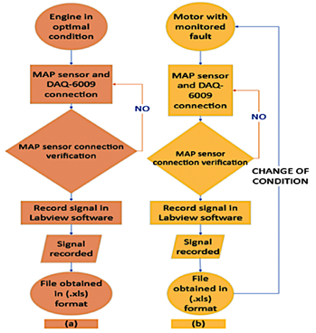
To acquire data from the MAP sensor signal, the systematized procedure shown in the flowchart in Figure 4 is followed.

The sampling methodology begins with the verification of the operating condition of the experimental unit, either under normal conditions or with supervised induced faults. The connection between the NI DAQ-6009 board and the MAP sensor of the MEP engine is then inspected. If the connection is correct, the signal is recorded in LabVIEW and the information is stored in an Excel file; otherwise, the connection is rechecked [1].

This procedure is applied identically to the MEP engine in optimal operating condition and to the engine with controlled faults, as shown in Figures 4(a) and 4(b) [1], [14]. Sample acquisition is repeated ten times for each condition defined in the experimental unit.

Figure 4. Flowchart for the sampling process: (a) engine under optimal conditions, (b) engine with induced fault

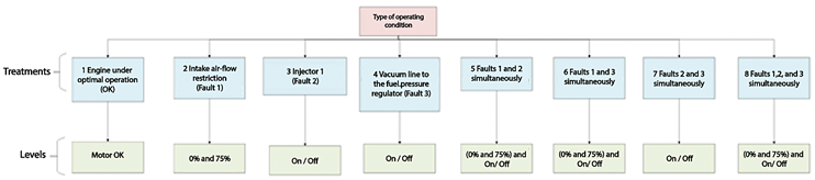
Figure 5 describes the eight operating conditions established for the engine under study, each with its corresponding level, including the optimal operating condition.

Figure 5. Functional states and operating levels defined for the MEP test unit

2.4.Extraction of MAP signal segments and selection of spectra to train the CNN

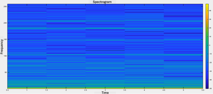
Spectrograms provide a visual representation of how a signal’s spectral content varies over time and are particularly effective for analyzing non-stationary signals. Accordingly, this study employs spectrograms to characterize the dynamic behavior of the MAP sensor signal.

To select the most suitable spectrograms for training the convolutional neural network (CNN), a script was first developed to segment each experimental treatment, comprising ten replicates, by dividing the MAP sensor signal into 250 fragments. An algorithm was then

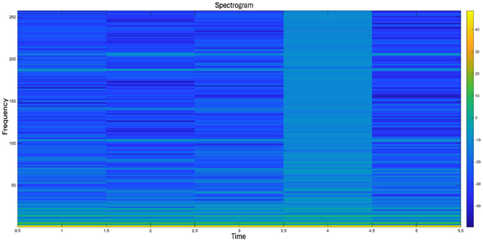
implemented in the MATLAB environment to automatically generate these representations, yielding 200 different spectrograms per treatment. The configuration used a sampling frequency of 10 kHz, a window size of 512 samples for spectral analysis, and an overlap of 128 samples between successive windows.

To determine the most suitable spectrograms to be used as input for the convolutional neural network (CNN), a detailed analysis of the 200 spectrograms generated for each treatment was performed, as shown in Figure 6. The region of lower-energy activity observed approximately between 3.5 and 4.5 s may indicate a transient condition, that is, an event associated with a disturbance in the MAP signal, as could occur under a fault condition in the MEP engine.

Figure 6. Example spectrogram from the set of 200 generate

From this process, the spectral pattern exhibiting the greatest consistency and representativeness was identified. Accordingly, 50 spectrograms per treatment that most faithfully reproduced this characteristic pattern were selected. Using MATLAB, the 50 spectrograms with the smallest mean distance from the average spectrum were selected as the most representative. This selection is supported by their ability to consistently

reproduce the characteristic spectro-temporal pattern of the MAP sensor under each operating condition.

Figure 7 shows the representative spectrogram corresponding to a sample of the engine under OK operating conditions. The horizontal axis represents time in seconds, while the vertical axis shows the distribution of spectral energy as a function of frequency from 0 to 250 Hz. This range encompasses the dominant variation of the intake-pressure pulse in Otto engines.

Figure 7. Representative spectrogram of the engine under OK operating conditions

The colorimetric map in Figure 7, expressed on dB scale, reflects the concentration of spectral power within each time–frequency region. Predominant energy is observed at low frequencies, below 40 Hz, associated with manifold-vacuum dynamics and the interaction between piston motion and the intake system. The periodic variations distributed over time indicate the cyclical consistency of the MAP signal under stable operating conditions. Localized variations in the intermediate bands, approximately 80 to 180 Hz, are related to fluctuations in volumetric filling.

2.5.Convolutional neural network (CNN) model

Using Python in the Visual Studio Code development environment, a convolutional neural network (CNN)–based algorithm was developed. This architecture belongs to the field of deep learning, a branch of machine learning characterized by its capacity to learn autonomously from large datasets. Its main strength lies in detecting complex patterns in images, which makes CNNs particularly suitable for classification and recognition tasks.

The use of a CNN is fully justified by the spectral, two-dimensional nature of the data obtained from the MAP sensor. By transforming the time-domain signal

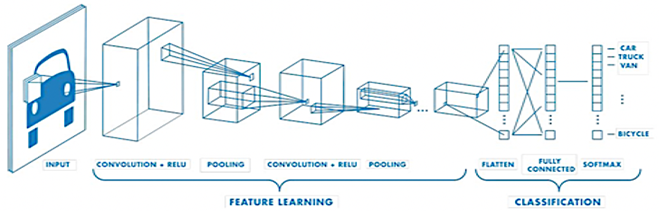
into spectrograms, the relevant engine information is encoded in time–frequency energy patterns that exhibit complex structures. Such patterns cannot be captured adequately by traditional models such as SVMs, decision trees, or fully connected neural networks.

CNNs, owing to their architecture based on convolutional filters, enable automatic extraction of hierarchical spatial features from spectrograms, thereby

identifying subtle variations associated with pressure dynamics, combustion irregularities, and fault-related effects in the intake, injection, or ignition systems. Because the model input consists of images, CNNs represent the standard approach for processing this type of data. Unlike feed-forward ANNs or models based on SVM or Random Forest, CNNs learn directly from the spectrograms through convolutional filters that capture high-frequency patterns, concentrated energy regions, and temporal structures corresponding to different fault modes.

Figure 8 presents the CNN architecture, in which images are processed through filters applied across successive convolutional layers. Each layer extracts progressively more complex features, enabling a hierarchical representation of the relevant information and facilitating interpretation of the visual content.

Figure 8. Convolutional neural network (CNN) architecture [20]

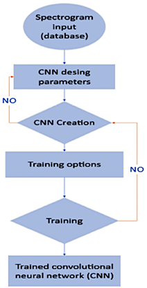
The proposed CNN architecture, consisting of three convolutional layers followed by pooling and dense layers, learns complex patterns without overfitting and with reasonable training times. The results yield an MSE below 1%, outperforming traditional ANN models that operate on less processed MAP signals.

Figure 9 presents the flowchart describing the convolutional neural network (CNN) training process, specifically designed to predict exhaust gas emissions and detect potential faults in the evaluated experimental unit.

Figure 9. Flowchart of the CNN training process

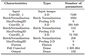
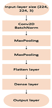
The algorithm begins by reading of the spectrogram database, after which the images are normalized by dividing their values by 255, thereby scaling them to the range from 0 to 1. Then, the dataset is divided into two subsets: 70 % is allocated for model training, and the remaining 30 % is reserved for testing.

Once these steps are completed, the initial parameters of the convolutional neural network (CNN) are configured, including the input-layer size, defined as (224, 224, 3), which corresponds to the dimensions of the images used. In the following stages, the CNN architecture is constructed with three convolutional layers, each followed by its corresponding normalization layer and dimensionality-reduction layers using MaxPooling2D.

Additionally, the network incorporates fully connected layers and a final regression layer responsible for estimating the exhaust-gas values, as presented in Table 3.

Table 3. Characteristics of the CNN architecture

Figure 10 illustrates the convolutional neural network developed to predict pollutant emissions in Otto engines using spectrograms derived from the MAP sensor signal. The architecture begins with an input layer that receives 224 × 224 × 3 images, followed by three sequential Conv2D–Batch Normalization – MaxPooling2D blocks that extract and progressively reduce the dimensionality of the time–frequency features contained in the spectrograms.

Subsequently, the network includes a flatten layer that converts the feature maps into a one-dimensional vector, which is then processed by a dense (fully connected) layer and fed to an output layer implementing multivariable regression to generate the predictions. This configuration enables efficient hierarchical extraction of relevant patterns for accurate estimation of CO, CO₂, HC, and O₂ emissions.

For training, the Adam optimizer was used with 50 epochs and a batch size of 16 samples.

Figure 10. Structure of the proposed CNN

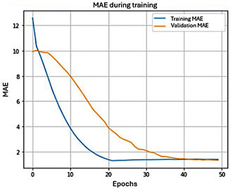
At the end of this stage, model performance was evaluated by calculating the mean squared error (MSE). This evaluation was complemented with graphica analyses, including a scatter plot, an error histogram, and a point-by-point comparison plot, which enabled a more detailed assessment of the model’s accuracy.

Subsequently, the prediction error was estimated for each output corresponding to CO, HC, CO₂, and O₂ emissions. When the error exceeded the 5% threshold, the model parameters were adjusted to improve predictive accuracy.

Figure 11 presents the results obtained using the mean absolute error (MAE) metric, which was used to evaluate the regression model’s performance. This metric quantifies the absolute difference between the CNN-predicted values and the corresponding groundtruth values. After training for 50 epochs with a maximum of 900 iterations, the model achievedMSE values of 0.1294 % for CO, 0.0200 % for HC, 0.0320 % for CO₂, and 0.0100 % for O₂.

Figure 11. Mean absolute error (MAE) during CNN training

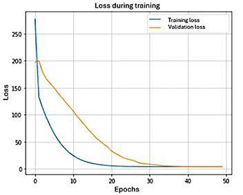
Figure 12 shows the variation of the loss during the convolutional neural network (CNN) training. As expected for this type of network, the loss begins at a relatively high level and decreases rapidly as the model adjusts to the data. This sustained downward trend indicates that the network is learning effectively and progressively optimizing parameters throughout the training process.

Figure 12. Loss curve during CNN training

3. Results and discussion

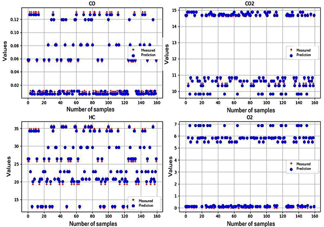
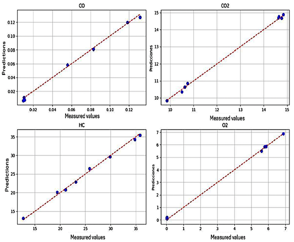
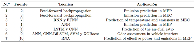
To evaluate the model’s performance in predicting fault-associated emissions from components and actuators, several tests were conducted using different analysis methods. Figure 13 illustrates 160 records from the testing phase. In this plot, blue circles denote the values estimated by the convolutional neural network (CNN), whereas red crosses indicate the corresponding measured values. As observed, the model’ predictions are highly accurate, with errors not exceedin 1% in any case. In addition, the mean absolute error (MAE) and mean squared error (MSE) were computed, and their resulting values confirm the reliability and appropriate fit of the proposed model.

Figure 14 compares the measured values with the predictions produced by the convolutional neural network (CNN) for CO, CO₂, HC, and O₂ concentrations. The blue points, representing the model estimates, cluster closely around the reference line, indicating accurate emission prediction across different operating conditions. In addition, the network correctly discriminated the eight operating conditions of the sparkignition engine (MEP), supporting the robustness of the proposed model.

Table 4 summarizes representative automotive applications that employ various techniques for emission prediction, together with the key factors associated with each approach.

Figure 13. CNN estimation results for exhaust-gas emissions CO, CO₂, HC, O₂

Figure 14. CNN prediction results for CO, CO₂, HC, and O₂ emissions

Table 4. Related studies on emission prediction in the automotive field

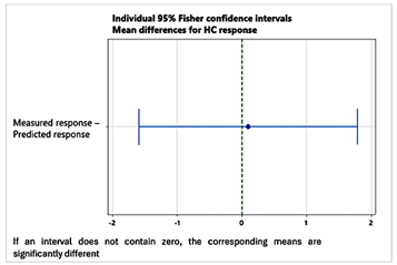
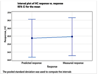
The results confirm that the proposed methodology is effective for both fault diagnosis and pollutantemission prediction. The close agreement between measured values and model estimates indicates that the approach can accurately identify the engine operating state and compute exhaust-gas concentrations with a minimal margin of error.

In [2], neural networks were developed to predict CO and HC, yielding errors of 5.40e-9 and 9.75e-5, respectively. Likewise, the study in [1] reports comparably low prediction errors and an excellent fit for CO₂ estimation, with a coefficient of determination (R²) of 99.2% and reduced RMSE and MSE values. In addition, the application of artificial neural networks has enabled accurate prediction of engine performance parameters and emissions, such as NO_x and HC, as demonstrated in [10], where accuracies of 99 % and 98 % were achieved, respectively.

Therefore, the results indicate that the proposed methodology, based on MAP signal spectrograms and a convolutional neural network (CNN) , achieves remarkable accuracy in the simultaneous estimation of pollutant emissions (CO, CO₂, HC, and O₂), with errors below 1 %. These values substantially outperform those reported in previous studies using traditional techniques such as fully connected neural networks (ANNs), support vector machines (SVMs), or multivariate regression–based methods, as summarized in Table 4.

Figure 15 presents a statistical analysis of the grouped data, comparing the real operating condition of the experimental unit with the concentrations of unburned hydrocarbons (HC) predicted by the convolutional neural network (CNN). The comparison was performed using Tukey’s test at a 95 % confidence level.

Figure 16 shows an interval plot comparing measured HC concentrations with the values estimated by the convolutional neural network (CNN). The results reveal no statistically significant differences among the mean values under the different operating conditions of the spark-ignition engine (MEP), thereby reinforcing the model’s reliability across diverse operating scenarios

Figure 15. Comparative mean plot of measured HC values and CNN predictions

Figure 16. Interval plot comparing measured HC values and CNN predictions

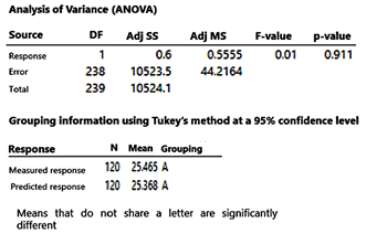
Figure 17 similarly analyzes the relationship between the values estimated by the convolutional neural network (CNN) and the measured values, applying Tukey’s test to assess potential differences. The results show that both sets share the same grouping letter (A), indicating no statistically significant differences between them.

Additionally, the analysis of variance (ANOVA) yielded a p-value of 0.911, which supports the consistency and accuracy of the developed model.

Figure 17. ANOVA results and Tukey’s test for measured and CNN-predicted values

3.1.Limitations

This study was conducted on an Otto engine equipped with a modern injection system, within a specific range of operating points and induced fault types. This choice reflects the need for a controlled environment that isolates the effect of faults on emissions and enables CNN training with consistent, repeatable data. Accordingly, the results are representative and robust for the engine and conditions considered, and they demonstrate the potential of the proposed methodology to link component and actuator faults with variations in emissions.

4. Conclusions

This study integrates data acquisition systems with artificial intelligence algorithms to enable early fault diagnosis in spark-ignition engines (MEP). The analysis focused on anomalies in the vacuum line of the fuel pressure regulator and in the air filter. The proposed method detects faults without dismantling components, thereby providing a minimally invasive diagnostic approach.

Experimental tests confirmed that the CNN-based model, comprising three convolutional layers with normalization and MaxPooling2D, achieves high accuracy in predicting emissions. Low mean squared error (MSE) values were obtained: 0.1294 % for CO, 0.0200 % for HC, 0.0320 % for CO₂, and 0.0100 % for O₂, using 50 training epochs and up to 900 iterations.

In addition, a one-way analysis of variance was performed in Minitab, yielding a p-value of 0.911. This result indicates no statistically significant difference

between the measured values and those estimated by the network, supporting the model’s reliability.

Overall, these findings highlight the potential of convolutional neural networks as an effective, noninvasive solution for fault detection and emission prediction in spark-ignition engines. The proposed approach achieves a low margin of error and demonstrates practical applicability in internal combustion systems.

Although the metrics used (MSE and MAE) are sufficient to demonstrate the accuracy of the convolutional model, additional indicators may add value in comparative or sensitivity analyses. Therefore, future work should incorporate metrics such as RMSE, R², and MAPE.

Contributor role

· Elmer I. Arias-Montaño: conceptualization, data curation, formal analysis, investigation, methodology, project administration, resources, software, supervision, validation, visualization, writing – original draft, writing – review & editing.

· Rogelio S. León-Japa: conceptualization, formal analysis, investigation, methodology, project administration, resources, software, supervision, validation, visualization, writing – review & editing.

· Pedro García-Jaramillo: data curation, software, validation.

· José Maldonado-Ortega: data curation, software, validation.

References

[1] W. R. Contreras Urgiles, R. S. León Japa, and J. L. Maldonado Ortega, “Predicción de emisiones de co y hc en motores otto mediante redes neuronales,” Ingenius, no. 23, pp. 30–39, Dec. 2019. [Online]. Available: https://doi.org/10.17163/ings.n23.2020.03

[2] F. Narváez, F. E. Sierra Vargas, and M. A. Montenegro Mier, “Modelo basado en redes neuronales para predecir las emisiones en un motor diésel que opera con mezclas de biodiésel de higuerilla,” Informador Técnico, vol. 76, p. 46, Dec. 2012. [Online]. Available: https://doi.org/10.23850/22565035.28

[3] R. S. Chauhan and N. Shrivastava, “Neuro fuzzy-grey wolf optimization-based modelling and analysis of diesel engine using tire oil with different proportions

of 2-ehn,” Fuel, vol. 384, p. 133849, Mar. 2025. [Online]. Available: https://doi.org/10.1016/j.fuel.2024.133849

[4] F. Sapio, F. Aglietti, P. Ferreri, and A. Savuca, “Neural-network-based modeling of scr systems for emission simulation: A comprehensive approach,” SAE International Journal of Advances and Current Practices in Mobility, vol. 07, no. 3, pp. 1437–1452, Sep. 2024. [Online]. Available: https://doi.org/10.4271/2024-24-0042

[5] H. H. Imtiaz, P. Schaffer, Y. Liu, P. Hesse, A. Bergmann, and M. Kupper, “Qualitative and quantitative analyses of automotive exhaust plumes for remote emission sensing application using gas schlieren imaging sensor system,” Atmosphere, vol. 15, no. 9, p. 1023, Aug. 2024. [Online]. Available: https://doi.org/10.3390/atmos15091023

[6] W. Torres Guin, J. Sánchez Aquino, S. Bustos Gaibor, and M. Coronel Suarez, “Arquitectura de iot para el monitoreo de emisiones de gases contaminantes de vehículos y su validación a través de machine learning,” Ingenius, no. 32, pp. 9–17, Oct. 2024. [Online]. Available: https://doi.org/10.17163/ings.n32.2024.01

[7] R. S. Jawad and H. Abid, “Hvdc fault detection and classification with artificial neural network based on aco-dwt method,” Energies, vol. 16, no. 3, p. 1064, Jan. 2023. [Online]. Available: https://doi.org/10.3390/en16031064

[8] F. Ricci, M. Avana, and F. Mariani, “Enhancing lambda measurement in hydrogen-fueled si engines through virtual sensor implementation,” Energies, vol. 17, no. 16, p. 3932, Aug. 2024. [Online]. Available: https://doi.org/10.3390/en17163932

[9] D. Tian, Q. Li, F. Liu, J. Khan, M. Q. Abbas, and Z. Du, “Voc data-driven evaluation of vehicle cabin odor: from ann to cnn-bilstm,” Environmental Science and Pollution Research, vol. 31, no. 22, pp. 32 826–32 841, Apr. 2024. [Online]. Available: https://doi.org/10.1007/s11356-024-33293-y

[10] I. Cesur and F. Uysal, “Experimental investigation and artificial neural network-based modelling of thermal barrier engine performance and exhaust emissions for methanol-gasoline blends,” Energy, vol. 291, p. 130393, Mar. 2024. [Online]. Available: https://doi.org/10.1016/j.energy.2024.130393

[11] A. K and P. Rithishbrahma, “Prediction of vehicle carbon emission using machine learning,” in 2024 5th International Conference on Electronics and Sustainable Communication Systems (ICESC). IEEE, Aug. 2024, pp. 1814–1818. [Online]. Available: https://doi.org/10.1109/ICESC60852.2024.10690134

[12] M. A. Rahim, M. M. Rahman, M. S. Islam, A. J. M. Muzahid, M. A. Rahman, and D. Ramasamy, “Deep learning-based vehicular engine health monitoring system utilising a hybrid convolutional neural network/bidirectional gated recurrent unit,” Expert Systems with Applications, vol. 257, p. 125080, Dec. 2024. [Online]. Available: https://doi.org/10.1016/j.eswa.2024.125080

[13] H. Sun and P. Chen, “Application of neural networks in automotive engine misfire,” in 2024 IEEE 4th International Conference on Electronic Communications, Internet of Things and Big Data (ICEIB). IEEE, Apr. 2024, pp. 261–264. [Online]. Available: https://doi.org/10.1109/ICEIB61477.2024.10602668

[14] M. Abboush, D. Bamal, C. Knieke, and A. Rausch, “Intelligent fault detection and classification based on hybrid deep learning methods for hardware-in-the-loop test of automotive software systems,” Sensors, vol. 22, no. 11, p. 4066, May 2022. [Online]. Available: https://doi.org/10.3390/s22114066

[15] S.-C. Lin, S.-F. Su, and Y. Huang, “A time-frequency signal-based convolutional neural network algorithm for fault diagnosis of gasoline engine fuel control system,” in 2019 International Conference on System Science and Engineering (ICSSE). IEEE, Jul. 2019, pp. 81–87. [Online]. Available: https://doi.org/10.1109/ICSSE.2019.8823285

[16] A. Maged and M. Nour, “Prediction of combustion pressure with deep learning using flame images,” Fuel, vol. 380, p. 133203, Jan. 2025. [Online]. Available: https://doi.org/10.1016/j.fuel.2024.133203

[17] Z. Li, Z. Qin, W. Luo, and X. Ling, “Gasoline engine misfire fault diagnosis method based on improved yolov8,” Electronics, vol. 13, no. 14, p. 2688, Jul. 2024. [Online]. Available: https://doi.org/10.3390/electronics13142688

[18] Y. Liu, J. Kang, L. Wen, Y. Bai, and C. Guo, “Health status assessment of diesel engine valve clearance based on bfa-boavmd adaptive noise reduction and multichannel information fusion,” Sensors, vol. 22, no. 21, p. 8129, Oct. 2022. [Online]. Available: https://doi.org/10.3390/s22218129

[19] W. R. Contreras Urgiles, J. Maldonado Ortega, and R. León Japa, “Aplicación de una red neuronal feed-forward backpropagation para el diagnóstico de fallas mecánicas en motores de encendido provocado,” Ingenius, no. 21, pp. 32–40, Dec. 2018. [Online]. Available: https://doi.org/10.17163/ings.n21.2019.03

[20] MathWorks. (2025) Redes neuronale convolucionales. The MathWorks, Inc. [Online]. Available: https://upsalesiana.ec/ing35ar7r20