Scientific Paper / Artículo Científico
		https://doi.org/10.17163/ings.n35.2026.05
		pISSN: 1390-650X / eISSN: 1390-860X
ANALYSIS OF CLOSED-FORM GROUND-RETURN IMPEDANCES FOR SHORT-CIRCUIT STUDIES IN OVERHEAD DISTRIBUTION SYSTEMS
ANÁLISIS DE IMPEDANCIAS DE TIERRA DE FORMA CERRADA EN ESTUDIOS DE CORTOCIRCUITO DE SISTEMAS DE DISTRIBUCIÓN AÉREA

Allen A. Castillo Barrón^1,* , Gerardo Ayala Jaimes¹ ,

Alejandra Jiménez Vega¹ , Francisco J. Ramírez Arias¹

Received: 29-04-2025, Received after review: 05-11-2025, Accepted: 18-11-2025, Published: 01-01-2026

Abstract	Resumen
The objective of this study is to evaluate the applicability of the most widely used closed-form groundreturn impedance formulas in short-circuit analyses of distribution systems and to identify the critical network configurations in which the choice of impedance model significantly affects the short-circuit results. The methodology adopted in this research is organized into three stages. First, an algorithm was developed to implement and compare several closed-form earthreturn impedance formulations, and its performance was validated using benchmark data reported in the literature. Second, a short-circuit analysis algorithm was designed and verified against reference results published by the IEEE Power and Energy Society. Finally, multiple short-circuit studies were performed on several IEEE distribution test feeders. The findings reveal that most closed-form earth-return impedance models provide adequate accuracy for both balanced and unbalanced short-circuit analyses. However, for single-phase line-to-ground faults, the choice of closedform impedance formulation is critical to obtaining accurate short-circuit results.	El objetivo de este estudio es evaluar la aplicabilidad de las principales fórmulas cerradas de impedancia de retorno por tierra en el análisis de cortocircuito de sistemas de distribución, así como identificar las configuraciones críticas en las cuales la elección del modelo de impedancia puede influir significativamente en los resultados del cortocircuito. La metodología adoptada en esta investigación se estructura en tres etapas. Primero, se desarrolló un algoritmo para implementar y comparar las formulaciones cerradas de impedancia de retorno por tierra, el cual fue validado con datos de referencia disponibles en la literatura. Segundo, se diseñó un algoritmo de análisis de cortocircuito que fue verificado con resultados publicados por la IEEE Power and Energy Society. Finalmente, se realizaron múltiples estudios de cortocircuito en varios alimentadores de prueba de distribución del IEEE. Los resultados muestran que la mayoría de las formulaciones cerradas de impedancia de retorno por tierra son adecuadas tanto para análisis de cortocircuito balanceados como desbalanceados, y que, en fallas monofásicas a tierra, la elección de la fórmula cerrada de impedancia resulta un factor crítico para obtener resultados precisos.
Keywords: Closed-form ground-return impedance, Distribution systems; Short-circuit calculation accuracy	Palabras clave: Fórmulas cerradas de impedancia de tierra, sistemas de distribución, exactitud de cálculo de cortocircuito

^1,*Department of Electrical Engineering (FCITEC), Universidad Autónoma de Baja California, Tijuana, México.

Corresponding author ✉: allen.castillo@uabc.edu.mx.

Suggested citation: A. A. Castillo Barrón, G. Ayala Jaimes, A. Jiménez Vega and F. J. Ramírez Arias “Analysis of closed-form ground-return impedances for short-circuit studies in overhead distribution systems,” Ingenius, Revista de Ciencia y Tecnología, N.◦ 35, pp. 64-77, 2026, doi: https://doi.org/10.17163/ings.n35.2026.05.

1. Introduction Distribution systems exhibit an inherently asymmetrical geometry and, unlike transmission lines, they are not transposed. This lack of symmetry leads to significant phase imbalances, increasing the current’s circulation through the earth. Consequently, accurately modeling the ground-return impedance is essential to obtaining a precise representation of the system’s electrical behavior [1–3]. The first model for earth-return impedance was developed by Carson in 1926, who derived the earliest analytical formulation by expressing the axial electric field in the soil as a Fourier-type improper integral under quasi-TEM assumptions. Carson’s model represents a foundational contribution to the field; however, it relied on simplifying assumptions such as homogeneous soil, ground permeability equal to that of free space, and the neglect of displacement currents, which limited its applicability at higher frequencies and in soils with significant permittivity effects [4]. Subsequent researchers addressed these limitations. Wise, in his early works from 1931 and 1934, introduced formulations that extended Carson’s model by incorporating finite ground permeability and displacement currents, using the Hertzian vector potential and Fourier–Bessel expansions to generalize the wave equation for imperfect soils [5,6]. Later, in 1968, Sunde further advanced Wise’s work by incorporating the effects of layered ground structures into the earth-return impedance formulations [7]. Carson’s formulation was originally expressed as improper integrals, which made its direct evaluation challenging. Over the years, researchers have proposed several methods to evaluate these integrals, including numerical integration techniques and infinite-series expansions [1], [8]. However, these approaches are often computationally intensive and require significant processing time. To address these limitations, multiple complex-image models have been developed. Sunde introduced a more rigorous physical basis for image placement and provided practical closed-form expressions [7]. Afterwards, Dubanton and Deri proposed more sophisticated complex-image depths derived from exponential or logarithmic approximations of Carson’s integral [9, 10]. Alvarado further refined these results by introducing a more accurate closed-form model suitable for engineering applications [11], while Pizarro and subsequently Noda presented double complex-image models in which two optimized image conductors substantially improve approximation accuracy across wide frequency ranges and geometric configurations [12, 13]. Finally, it is important to note that Kersting proposed a model that relies only on the first few terms of Carson’s series expansion [14], and that Carson himself, in his original work, had already derived

a closed-form solution, although this contribution remained largely unrecognized until recent years [15]. Closed-form solutions for ground-return impedance have been extensively studied, and numerous works have analyzed their sensitivity to soil resistivity, conductor height, horizontal spacing, operating frequency, and ground stratification. These studies provide valuable insights into the accuracy and limitations of both classical and modern approximations, including Carson-based series, image-method formulations, and recent closed-form expressions. However, despite this extensive body of research, no previous work has  evaluated the applicability or accuracy of these closedform models for short-circuit studies in unbalanced distribution systems, in which mutual coupling and asymmetrical feeder geometries significantly influence the results [1], [8], [16–18]. For short-circuit studies in balanced systems, the symmetrical components method is widely employed. However, in distribution networks, which are inherently unbalanced due to their asymmetrical geometry, directly applying this method can lead to significant errors [19]. In such cases, a phase-domain analysis becomes essential, as it explicitly represents system unbalance and incorporates the mutual impedances among phases. Recent studies have integrated phasedomain representations directly into the symmetrical components framework, enabling a more accurate treatment of unbalance and mutual coupling effects. These hybrid approaches are increasingly being used to analyze distribution systems with high penetration of distributed generation (DG), where the interaction between unbalanced network conditions and inverterbased resources necessitates detailed, phase-resolved short-circuit modeling [20–22]. Since short-circuit studies in distribution systems with distributed generation are now commonly performed using phase-domain analysis, which directly relies on an accurate representation of the earth-return impedance, it is essential to assess whether the most widely used closed-form formulations implemented in commercial software and research projects are suitable for this purpose [1], [17]. Evaluating their performance makes it possible to determine the reliability of these closed-form expressions for short-circuit calculations and, consequently, their appropriateness for analyzing unbalanced distribution systems with high DG penetration. This study provides a comprehensive phase-domain short-circuit analysis of three distribution systems, incorporating the most widely used closed-form formulations for ground-return impedance. The novelty of this study lies in evaluating, for the first time, the direct impact of these formulations on short circuit results in unbalanced distribution networks, rather than focusing

solely on their electromagnetic accuracy as in prior contributions.

The main contributions of this work are summa rized as follows:

· To quantify the percentage error introduced in short-circuit calculations when different closedfor ground-return impedance formulations are employed.

· To identify the critical network configurations in which the selection of the impedance model exerts a significant influence on short-circuit results.

2. Materials and Methods

2.1.Closed-form impedance formulas

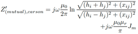
The principal closed-form expressions for earth-return impedance in overhead distribution lines are derived from Carson’s formulations [16, 17], [23] and include the following components:

(1)

Where R_c and X_c denote the conductor resistance and reactance, respectively, X_g represents the reactance associated with the geometric distribution of the conductors, and Z_e is the earth-return impedance. As is customary for short overhead lines (less than 50 miles), capacitance is neglected because it has a negligible impact at power frequencies [24].

The conductor resistance is typically provided by the manufacturer. The conductor reactance is given by:

(2)

Where

· ω is the complex frequency, rad/s.

· μ₀ is the vacuum permeability, H/mile.

· μ_r is the relative magnetic permeability.

· r_ext is the conductor radius, (ft).

· GMR is the geometric mean radius of the conductor, (ft).

The extended Carson model is presented in (3)-(6). In these expressions, Z_c denotes the conductor selfimpedance and is given by the sum of R_c and jX_c. The second term on the right-hand side of equation (3) and the first term on the right-hand side of equation (4)

correspond to the reactance associated with line geometry (jX_g). The last terms on the right-hand sides of (3) and (4) represent the earth-return impedance (Ze).

(3)

(4)

Where

(5)

(6)

And

· ρ is the ground resistivity, Ω · ft.

· h_s, h_i, h_j are the conductor heights above ground (ft).

· x is the horizontal separation between conductors (ft).

The solution to the infinite integrals in equations (5) and (6) was initially expressed by Carson as a closed-form solution. However, owing to the limited computational resources available at the time, he presented the result as an infinite-series expansion. Consequently, subsequent approximations became necessary to obtain practical formulations for earth-return impedance [1], [15]. This section summarizes the principal closed-form solutions for low frequencies, starting with the single- and double-logarithmic approximations to Carson’s integrals [9–13], followed by the computational adaptations of the corresponding infinite-series expressions [14], [23].

2.1.1. Dubanton

The first approximation considered in this study for the self-impedance of an overhead conductor was proposed by Dubanton in 1969, based on the concept of complex depth. Subsequently, in 1976, Gary derived an expression for the mutual impedance between two overhead conductors, thereby completing Dubanton’s formulation [9]. It is important to note that both expressions are empirical in nature.

(7)

(8)

where the complex depth (ft) is defined as:

(9)

2.1.2. Deri

In 1981, Deri et al. [10] provided a mathematical validation of the impedance formulas proposed by Dubanton and Gary. Their final closed-form solution is given by:

(10)

(11)

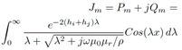
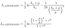
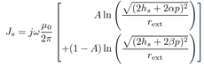
2.1.3. Alvarado

A year later, in 1982, Alvarado et al. improved the impedance formulas developed by Deri [11]. Their main contribution was proposing an approximation that retained more terms than Deri’s formulation. The resulting expression is given by:

(12)

(13)

(14)

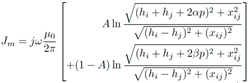
2.1.4. Pizarro and Eriksson

Pizarro and Eriksson [12] introduced a double logarithmic approach in 1991 to solve (3)-(6), as

summarized below:

(15)

(16)

Where the constants were obtained using the leastsquares method, yielding A = 0.1159, α = 0.2258 and β = 1.1015. These values are valid for both self and mutual impedance.

2.1.5. Noda

In 2006, Noda [13] extended the work of Pizarro and Eriksson by approximating A, α and β as functions of typical distribution- and transmission-system parameters, including frequency, ground resistivity, and conductor height. This refinement improved the accuracy of Pizarro’s impedance model; however, it required the introduction of an additional variable, θ.

The formulas for calculating self and mutual impedance are given in (15) and (16). The parameters A and α are defined as follows:

(17)

(18)

(19)

Where, for self-impedance, θ = 0◦, whereas for mutual-impedance calculations, it is given by:

(20)

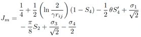
2.1.6. Galloway

Galloway’s impedance formulas [23] constitute a numerical adaptation of Carson’s complete series expansion and are expressed as follows:

(21)

(22)

Where γ denotes Euler’s constant (1.7811), and S₂, S′₂, S₄, S′₄, σ₁, σ₂, σ₃ and σ₄ are infinite series that are described in detail in [8].

And

(23)

(24)

for self-impedance calculations, D_ij = 2h_s.

Finally, the upper limit k in the summations was set to 35 , since Ramos et al. [17] showed that, for typical 60-Hz distribution-line configurations, retaining 35 terms in the Galloway formulas yields a deviation of less than 1×10−7 relative to the numerical evaluation of Carson’s integral. Accordingly, this work adopts the 35-term Galloway formulation as an exact numerical reference for Carson’s integral, denoted as the Carson model.

2.1.7. Kersting

Kersting’s formulas [14] are based on Carson’s recommendations for r less than 1/4 [4]. Most distributionline configurations under steady-state conditions (f = 60Hz) and with standard soil resistivity (ρ = 328.084 Ω · ft) fall within this range.

(25)

(26)

Finally, to obtain the phase-impedance matrix (Z) for all line models, Kron reduction must be applied to the corresponding primitive impedance matrix (Z´). The complete procedure is described in detail in [18].

2.2.Distribution Line Configurations

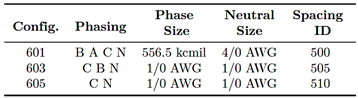
After presenting the closed-form earth-return impedance formulas, the next step is to model the line configurations for the short-circuit studies. To this end, an algorithm was developed in Mathematica software to incorporate all the earth-impedance formulations. The algorithm was then validated against benchmark data reported in the original references. Two distribution systems were selected for the studies. The IEEE 13-node test feeder was chosen because it is compact yet highly unbalanced, whereas the IEEE 34-node test feeder [25] was selected because it features long distribution lines. The test cases considered in this study are based on these IEEE test feeders, which were developed from actual distribution system configurations and are widely recognized as benchmark models for validating analysis methodologies in distribution networks. These feeders are now extensively used in short-circuit studies, phase-domain modeling, zero-sequence impedance evaluation, and analyses involving high DG penetration. Their broad adoption and sustained acceptance in recent literature support the representativeness and suitability of these configurations for the accuracy assessment conducted in this work [22], [26–28].

The IEEE 13-node test feeder includes five overhead line configurations (601–605); however, only three correspond to distinct conductor spacings. Accordingly, results are reported only for configurations 601, 603, and 605, which represent three-phase, two-phase, and single-phase lines, respectively. The principal data for these configurations are summarized in Table 1.

Table 1. Overhead line-configuration data for the IEEE 13-node test feeder

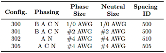
The IEEE 34-node test feeder includes four overhead line configurations. Configurations 300 and 301 are three-phase, configuration 305 is two-phase, and configuration 302 is single-phase. However, their conductor spacings are identical to those of the IEEE 13-node test feeder, as summarized in Table 2.

Table 2. Overhead line-configuration data for the IEEE 34-node test feeder

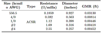
The conductor data for both systems are available in [25] and are summarized in Table 3. Conductor sizes are expressed in kcmil or AWG, and all conductors are of the ACSR type. Resistance values are reported in ohms per mile at 60 Hz and 50 °C. The conductor’s external diameter is given in inches, and the geometric mean radius (GMR) is expressed in feet.

Table 3. Conductor data

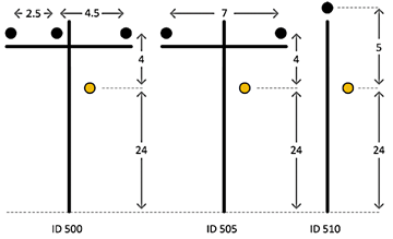
The configurations corresponding to the different spacings are illustrated in Figure 1, with all distances expressed in feet. Phase conductors are depicted in black, whereas the neutral conductor is shown in gold. The distance between the pole and the neutral conductor is 0.5 ft.

Figure 1. Line spacings

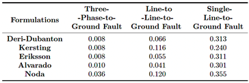
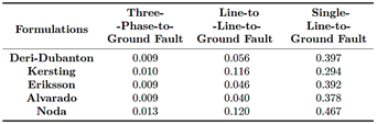
To properly assess the accuracy of the closed-form earth-return impedance formulas, Table 4 presents the maximum percentage error of the different impedance formulas relative to the Carson series for configurations 601, 603, and 605, corresponding to three-phase, two-phase, and single-phase cases, respectively. The modeling was performed at 60 Hz, assuming a soil resistivity of 100Ω ·m. This value was selected because typical soil resistivity ranges from 50 to 200Ω ·m, and 100Ω · m represents a moderately conservative condition for evaluating ground-return impedance behavior.

Moreover, 100Ω · m is widely used as a benchmark in recent academic studies and IEEE technical reports that assess image-based methods, Carson-derived models, and frequency-dependent impedance formulations [1], [8], [29,30]. The percentage error is computed as follows:

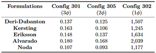
Table 4. Maximum percentage error for the different distribution-line configurations

(27)

It is important to emphasize that the Carson model is used as the reference in this work, since at low frequencies, there is no significant difference between the results obtained from Carson’s formulation and those obtained from Wise’s generalized earth-return impedance formula [6]. Wise’s model is regarded as the most comprehensive because it accounts for soil permeability and displacement currents. Nevertheless, at power frequencies, these displacement currents are negligible, and both formulations converge to essentially the same results [1].

From Table 4, it is evident that Noda’s formulas yield the smallest percentage errors in both the real and imaginary components. Alvarado’s formula provides the next most accurate approximation, with maximum percentage errors below 0.09%. Pizarro’s approximation follows, exhibiting, with a maximum error of 0.15% in two-phase configurations. In contrast, the Kersting and Deri formulas produce larger discrepancies, with maximum errors of approximately 0.32% and 1.19%, respectively. These findings are consistent with the conclusions drawn by Martins [16] and Ramos- Leaños [17], who identified Noda’s formulations as the most accurate closed-form approximation to the Carson series for typical distribution-line configurations. It is also worth noting that the procedure used in this study to compute percentage differences is identical to that adopted by Papadopoulos [1].

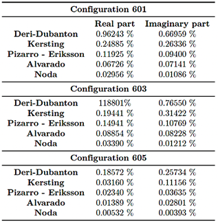
From these tables, it is evident that the Deri and Dubanton formulas yield identical impedance matrices for the line configurations analyzed in this study. Accordingly, they are combined and treated as a single formulation in the subsequent analysis.

Finally, it should be noted that the smallest percentage errors occur in the single-phase configurations (605). Moreover, because single-phase lines are typically short, these configurations are expected to exert only a limited influence on short-circuit calculations. In contrast, the two-phase configurations (603) exhibit larger percentage errors and, since such lines are generally of medium length, they are more likely to have a pronounced impact on short-circuit study results.

3. Results and discussion

This section presents the principal results of the shortcircuit studies conducted on the IEEE 13-node and 34-node test feeders. Three case studies are examined to represent distinct distribution-system conditions: a 13-bus feeder with short lines (less than 1 mile), a 34-bus feeder with long lines (up to 15 miles), and a third scenario characterized by extremely long lines (greater than 15 miles).

The algorithm used for these studies was implemented in Mathematica, and its results match exactly the reference data published by the IEEE Power and Energy Society [31]. Phase-domain analysis was adopted for the short-circuit calculations, since it is widely recognized as a benchmark approach for distribution-system studies [20], [27]. Detailed descriptions of this method are available in [32, 33]. Standard assumptions were applied throughout the short-circuit simulations: the pre-fault voltage was set to 1 pu, and static loads were neglected.

Before presenting the results of the short-circuit studies, it is important to clarify that, for ease of analysis, all outcomes are reported as the maximum percentage error, computed using equation (28). In this expression, I_Carson denotes the short-circuit current obtained with the Carson model, and I_{(E−formulae)} denotes the current obtained with the corresponding closed-form earth-impedance formulations. Short-circuit current values in amperes are available from the authors upon request.

(28)

The results for the different fault types are presented below. It is important to note that three-phase and line-to-line fault outcomes are not reported, since no significant differences were observed among the

impedance models. This behavior is expected because these faults do not involve an earth-return path; consequently, all formulations converge, resulting in essentially identical short-circuit current magnitudes.

3.1.IEEE 13-Node Test Feeder

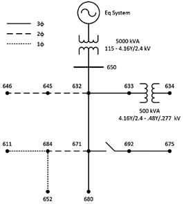
The first short-circuit study is conducted on the IEEE 13-node test feeder, whose one-line diagram is shown in Figure 2. In the diagram, solid, dashed, and dotted lines denote three-phase, two-phase, and single-phase line configurations, respectively.

Figure 2. IEEE 13-node test feeder

The complete system data is available in [31]. Table 5 summarizes the main line-segment data.

Table 5. Line-segment data for Case Study1

Segment 671–692 is not included in the table because it corresponds to a switch with zero length. The impedance matrices for the underground line segments 684-652 and 692-675 were taken from [31]. These matrices were kept unchanged, because their differences relative to the Carson model are less than 0.01% [34].

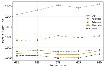
3.1.1. Three-Phase-to-Ground Fault Figure 3 presents the maximum percentage differences in short-circuit current between the Carson Model and the closed-form earth-impedance formulations for a three-phase-to-ground fault. Figure 3. Maximum percentage error for a three-phaseto- ground fault From Figure 3, it is evident that all closed-form impedance formulations yield errors below 0.006% for this fault type. Among them, Noda’s formulation provides the closest agreement with the Carson model, followed in decreasing accuracy by Alvarado, Eriksson, Kersting, and Deri. The largest percentage error occurs at node 680, which lies along the longest three-phase path from the short-circuit source, approximately 5000 ft. 3.1.2. Line-to-Line-to-Ground Fault Figure 4 depicts the maximum percentage errors in short-circuit current between the Carson model and the closed-form earth-impedance formulations for a line-to-line-to-ground fault. As Figure 4 shows, Noda’s formulations provide the closest agreement, followed by Alvarado’s and Eriksson’s. The Kersting and Deri formulations also perform well, with errors remaining below 0.05%. The highest average error occurs at node 680, which is located along the longest two-phase path from the short-circuit source (approximately 5000 ft). Notably, nodes 645 and 646 also exhibit relatively large errors because they are two-phase nodes; however, since the associated line sections are short, their overall effect remains limited.

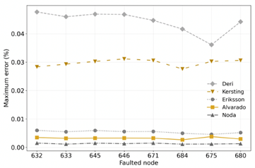
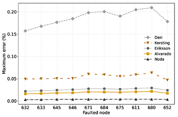
Figure 4. Maximum percentage error for a line-to-line toground fault 3.1.3. Single-Line-to-Ground Fault Figure 5 presents the maximum percentage differences in short-circuit current between the Carson model and the closed-form earth-impedance formulations for a single-line-to-ground fault. Figure 5. Maximum percentage error for a single-line-to- ground fault From Figure 5, it is evident that, for this fault type, all earth-impedance formulations yield errors below 0.21%. Consistent with the other fault cases, Noda’s formulation provides the closest agreement with the Carson model, followed closely by Alvarado’s and Eriksson’s, and then by Kersting’s and Deri’s. 3.1.4. Analysis for Case Study 1 Based on the short-circuit results, it can be concluded that the largest discrepancies generally occur for singleline-

to-ground faults (0.21%), followed by line-to-lineto- ground faults (0.05%), and, finally, three-phase-toground faults (0.006%). Across all fault types, Noda’s formulation provides the most accurate approximation, closely followed by Alvarado’s and Eriksson’s. The remaining earth-impedance formulations introduce errors that may be non-negligible in certain applications, particularly when longer line sections are involved. An updated analysis is conducted to examine the relationship between the modeling errors associated with the line configurations and the errors observed in the short-circuit studies, with the aim of determining whether a correlation exists between these parameters. Because node 680 exhibits the largest short-circuit error and configuration 601 connects the source node (650) to node 680, the assessment focuses on the threephase configuration 601. For this configuration, the reactive component is approximately three times larger than the resistive component; therefore, the imaginary part is adopted as the reference for the correlation analysis. Table 6 summarizes the relationship between impedance-modeling errors, and the maximum shortcircuit errors at node 680. The reported values are obtained by dividing the maximum short-circuit errors by the maximum errors in the imaginary part of the corresponding impedances, so that larger ratios indicate a stronger correlation. Table 6. Relationship between impedance errors and shortcircuit results From Table 6, it can be concluded that impedancemodeling errors exert a stronger influence on lineto-ground faults, as reflected by the larger ratios. It should be noted that this assessment was performed only for node 680, which is a three-phase node. A more comprehensive understanding requires extending the same analysis to two-phase and single-phase nodes associated with longer line sections. This extended evaluation is addressed in the following cases. 3.2. 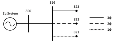Long distribution lines The objective of this case study is to examine how line length affects the magnitude of short-circuit fault currents. The short-circuit analysis is performed on a section of the IEEE 34-node test feeder, as shown in the

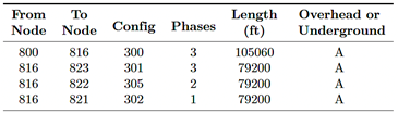
one-line diagram in Figure 6. In the diagram, solid, dashed, and dotted lines denote three-phase, two-phase, and single-phase line configurations, respectively. Figure 6. IEEE 34-nodetest feeder The main feeder section up to node 816 is modeled as a three-phase line with configuration 300 and a length of 105,060 ft. From node 816 onward, three branches are considered: a three-phase branch with configuration 301, a two-phase branch with configuration 305, and a single-phase branch with configuration 302. The key line-segment data are summarized in Table 7. Table 7. Line-segment data for Case Study 2 The results are presented for terminal nodes located 3, 6, 9, 12, and 15 miles downstream from the three-phase node 816. 3.2.1. Three-Phase-to-Ground Fault Figure 7 depicts the maximum percentage differences in short-circuit current between the Carson model and the closed-form earth-impedance formulations for a three-phase-to-ground fault at node 823. Figure 7. Maximum percentage error for a three-phaseto- ground fault in Case Study2 (node 823)

From Figure 7, it is evident that all closed-form formulations yield errors below 0.005% for this fault type. 3.2.2. Line-to-Line-to-Ground Fault Figure 8 depicts the maximum percentage error in short-circuit current between the Carson model and the closed-form earth-impedance formulations for a line-to-line-to-ground fault, corresponding to the twophase case. Figure 8. Maximum percentage error for a line-to-line toground fault in Case Study 2 (node 822, two-phase) The three-phase case is not reported because it is essentially identical to the two-phase case; both exhibit a maximum error of 0.05% for the Deri formulation. 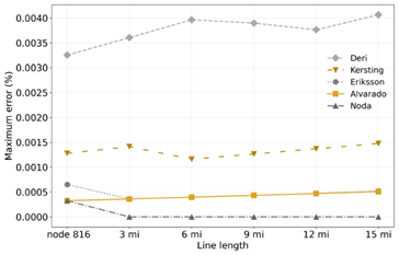3.2.3. Single-Line-to-Ground Fault Figure 9 depicts the maximum percentage differences in short-circuit current between the Carson model and the closed-form earth-impedance formulations for a single-line-to-ground fault, corresponding to the singlephase case. Figure 9. Maximum percentage error for a single-line toground fault in Case Study 2 (node 821, single-phase) From Figure 9, it is evident that Noda’s formulations provide the closest agreement with the Carson model, followed by Alvarado’s, Eriksson’s, and Kersting’s. The Deri formulations also perform satisfactorily, with errors remaining below 0.18%. It should be noted that the three-

phase and two-phase cases exhibit trends comparable to those of the single-phase configuration; therefore, they are not reported. 3.2.4. Analysis for Case Study 2 Based on the short-circuit results, it can be concluded that the largest discrepancies generally occur for singleline- to-ground faults (0.19%), followed by double lineto- ground faults (0.05%), and, finally, three-phase-toground faults (0.005%). Across all fault types, Noda’s formulations provide the most accurate approximation, closely followed by the Alvarado and Eriksson methods. The remaining formulations exhibit errors that may be non-negligible in line-to-earth fault calculations. After analyzing the results of the first and second case studies, it is apparent that the line-to-ground fault constitutes the most critical scenario. Accordingly, a correlation analysis is conducted to examine the relationship between line-modeling errors and the outcomes of the line-to-ground fault studies. For configurations 302 and 305, which correspond to single-phase and two-phase lines, the resistive component is approximately twice the reactive component; therefore, these configuration are adopted as the reference cases for this assessment. Table 8 summarizes the relationship between linemodeling errors and the maximum errors obtained in the short-circuit studies at a distance of 15 miles from node 816. The values reported in Table 8 are computed as the ratio of the maximum short-circuit errors to the maximum errors in the real part of the corresponding impedances. Larger values indicate a stronger correlation. Table 8. Relationship between impedance-modeling error and line-to-earth short-circuit results From Table 8, it can be concluded that impedancemodeling error is most influential in the single-phase configuration, as evidenced by the larger ratios. This indicates a close relationship between line-modeling error and line-to-ground fault error for single-phase lines. Regarding the three-phase and two-phase configurations, the influence of modeling error on short-circuit calculations also remains significant, consistent with the findings of Case Study 1; nevertheless, the singlephase configuration continues to represent the critical case. Finally, to encompass all relevant operating conditions, extremely long lines must be considered, and this scenario is examined in the final case study.

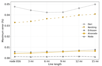
3.3. Very long distribution lines The objective of this third case study is to examine short-circuit fault magnitudes in extremely long distribution lines (greater than 50 miles), thereby covering all relevant scenarios in distribution-system modeling. Figure 10 illustrates the system adopted for this analysis, which is based on the IEEE 13-node test feeder. Specifically, the overhead line section between nodes 650 and 632 is extended to a total length of 50 miles. This line uses the three-phase configuration 601, with parameters provided in Table 1. Only the three-phase case is considered, since extremely long distribution lines are typically implemented using three-phase configurations. 3.3.1. 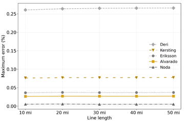Short-circuit results Figure 10 illustrates the maximum percentage differences in short-circuit current between the Carson model and the closed-form earth-impedance formulations for a single line-to-ground fault. From Figure 10, it is evident that Noda’s formulations provide the closest agreement with the Carson model, followed by Alvarado’s, Eriksson’s, and Kersting’s. The Deri formulations also perform satisfactorily, with errors remaining below 0.27%. The results for the three-phase-to-ground and double line-to-ground faults are not reported because they exhibit behavior similar to that shown in Figures 7 and 8 for Case Study 2. The maximum percentage error is 0.007% for the three-phase-to-ground fault and 0.04% for the double line-to-ground fault. Figure 10. Maximum percentage error for a single-lineto- ground fault in Case Study 3. 3.3.2. Analysis for Case Study 3 The three-phase-to-ground fault study shows that all closed-form earth-impedance formulations yield maximum errors below 0.007%. A consistent trend

emerges when these results are compared with those of Case Studies 1 and 2. Specifically, Case Study 1 reported a maximum error of 0.006% at 1 mile from the source, whereas Case Study 2 showed a maximum error of 0.005% at 15 miles. Collectively, these findings indicate that the closed-form earth-impedance formulations considered are sufficiently accurate for modeling three-phase-to-ground faults. For line-to-line-to-ground faults, all closed-form earth-impedance formulations exhibit maximum errors of approximately 0.04%. This result is consistent with Case Studies 1 and 2, which reported maximum errors of 0.05% at 2000 ft and 15 miles, respectively. Across all cases, the maximum error remains below 0.05%, indicating that the closed-form earth-impedance formulations considered are sufficiently accurate for modeling this fault type. For line-to-earth (single-line-to-ground) faults, all closed-form earth-impedance formulations exhibit maximum errors of 0.27%. Case Study 1 reported a maximum error of 0.21% at 5000 ft, whereas Case Study 2 showed a maximum error of 0.19% at 15 miles. Across all three case studies, the maximum error remains below 0.27%. Based on the results of this short-circuit study, it can be concluded that the largest discrepancies generally occur for line-to-ground faults (0.27%), followed by double line-to-ground faults (0.04%), and, finally, threephase-to-ground faults (0.007%). Among the evaluated formulations, Noda’s model provides the most accurate approximation across all fault types, closely followed by those of Alvarado and Eriksson. By contrast, the remaining formulations may introduce non-negligible errors in line-to-earth fault calculations, particularly in applications that demand high accuracy. These conclusions are consistent with the trends observed in the previously analyzed case studies and are directly relevant to ongoing research examining the influence of distributed generation on short-circuit current magnitudes [22], [35, 36]. A correlation analysis is conducted to examine the relationship between line-modeling error magnitudes and the outcomes of the short-circuit studies. For configuration 601, the reactive component is approximately three times larger than the resistive component; therefore, the reactive part is adopted as the reference for this assessment. Table 9 presents the relationship between line-modeling errors, and the maximum shortcircuit errors observed at a distance of 50 miles from node 650. The values reported in Table 9 are computed by dividing the maximum short-circuit errors by the maximum modeling errors associated with the reactive part of the corresponding impedances.

Table 9. Relationship between impedance-modeling error and short-circuit results From Table 9, it can be concluded that impedancemodeling errors are most consequential for line-toground faults, as evidenced by the strong correlation observed for most closed-form earth-impedance formulations. By contrast, for three-phase and lineto- line faults, no clear relationship emerges between impedance-modeling errors and short-circuit results. Accordingly, for very long distribution lines, the choice of earth-impedance formulation has a negligible influence on short-circuit calculations under these fault conditions. 4. Conclusions This study presented, in a comprehensive and accessible manner, the most widely used closed-form earth-return impedance formulations for short-circuit analysis in distribution systems. These formulations were applied to model single-phase, two-phase, and three-phase line configurations representative of practical distribution networks. Their impedance accuracy was quantified through percentage-error comparisons against the Carson reference model. After the line-modeling stage, three short-circuit case studies were conducted. The first examined a feeder with short lines (less than 1 mile), the second considered medium-length lines (up to 15 miles), and the third evaluated very long lines (up to 50 miles). In each case, the percentage error between short-circuit currents computed using closed-form formulations and those obtained with the Carson model was determined. Across all studies, line-to-ground faults consistently produced the largest percentage errors, followed by line-to-line-to-ground faults, whereas three-phase-toground faults exhibited the smallest errors. Notably, three-phase and line-to-line faults exhibited negligible differences between the studied formulations and the Carson model. For all cases, the maximum error for three-phaseto- ground faults remained below 0.007%, and for lineto- line-to-ground faults below 0.04%, confirming that all closed-form formulations considered are adequate for modeling these fault categories. In contrast, line-to-ground faults reached a maximum error of 0.27%,

indicating that the selection of the earth-return impedance formulation can be consequential in studies where high short-circuit accuracy is required. Among the evaluated formulations, Noda’s model consistently provided the most accurate approximation to the Carson reference, closely followed by Alvarado’s and Eriksson’s formulations, while Kersting’s and Deri’s yielded the largest deviations. In general, formulations with more elaborate complex-image representations tended to achieve higher accuracy. Nevertheless, except for line-to-ground faults, simpler formulations appear sufficient for short-circuit studies and may be preferred when reducing computational effort is a priority. The correlation analysis further showed that, for three-phase and line-to-line-to-ground faults, impedance-modeling errors do not translate into noticeable short-circuit calculation errors. By contrast, a strong correlation was observed for line-to-ground faults, particularly in single-phase configurations, underscoring that accurate earth-return impedance modeling is critical in these scenarios. Overall, the closed-form earth-return impedance formulations investigated are suitable for short-circuit analysis in distribution systems. However, for singleline- to-ground faults in single-phase lines, the choice of closed-form formulation is crucial to ensuring accurate short-circuit results. Contributor Roles · Allen A. Castillo Barrón: Conceptualization, formal analysis, methodology, project administration, writing – original draft and writing – review & editing. · Gerardo Ayala Jaimes: Resources, software, visualization, writing – original draft and writing – review & editing. · Alejandra Jiménez Vega: Investigation, supervision and validation. · Francisco J. Ramírez Arias: Data curation, software and visualization. References [1] T. A. Papadopoulos, A. I. Chrysochos, C. K. Traianos, and G. Papagiannis, “Closed-form expressions for the analysis of wave propagation in overhead distribution lines,” Energies, vol. 13, no. 17, p. 4519, Sep. 2020. [Online]. Available: https://doi.org/10.3390/en13174519

[2] R. Cleenwerck, H. Azaioud, R. Claeys, T. Coosemans, J. Knockaert, and J. Desmet, “An approach to the impedance modelling of low-voltage cables in digital twins,” Electric Power Systems Research, vol. 210, p. 108075, Sep. 2022. [Online]. Available: http://doi.org/10.1016/j.epsr.2022.108075 [3] J. Zhang, F. Geth, R. Heidari, and G. Verbič, “Beyond simplifications: Evaluating assumptions for low-voltage network modelling in the der era,” Sustainable Energy, Grids and Networks, vol. 43, p. 101860, Sep. 2025. [Online]. Available: http://doi.org/10.1016/j.segan.2025.101860 [4] J. R. Carson, “Wave propagation in overhead wires with ground return,” Bell System Technical Journal, vol. 5, no. 4, pp. 539–554, Oct. 1926. [Online]. Available: http://doi.org/10.1002/j.1538-7305.1926.tb00122.x [5] W. H. Wise, “Effect of ground permeability on ground return circuits,” Bell System Technical Journal, vol. 10, no. 3, pp. 472–484, Jul. 1931. [Online]. Available: http://doi.org/10.1002/j.1538-7305.1931.tb01287.x [6] W. Wise, “Propagation of high-frequency currents in ground return circuits,” Proceedings of the IRE, vol. 22, no. 4, pp. 522–527, Apr. 1934. [Online]. Available: http://doi.org/10.1109/JRPROC.1934.225868 [7] E. D. Sunde, Earth Conduction Effects in Transmission Systems. Dover Publications, 1968. [Online]. Available: https://upsalesiana.ec/ing35ar5r7 [8] H. Wohlfarth, “Calculation of ground impedances,” IEEE Transactions on Pow Delivery, vol. 39, no. 4, pp. 2113–2124, Aug. 2024. [Online]. Available: https://doi.org/10.1109/TPWRD.2024.3388570 [9] C. Dubanton, “Calcul approché des parametres primaires et secondaires d’une ligne de transport,” EDF Bulletin de la Direction des Études et Recherches, no. 1, pp. 53–62, 1969, cited by: 16. [Online]. Available: https://upsalesiana.ec/ing35ar5r10 [10] A. Deri, G. Tevan, A. Semlyen, and A. Castanheira, “The complex ground return plane a simplified model for homogeneous and multi-layer earth return,” IEEE Transactions on Power Apparatus and Systems, vol. PAS-100, no. 8, pp. 3686–3693, Aug. 1981. [Online]. Available: https://doi.org/10.1109/TPAS.1981.317011

[11] F. Alvarado and R. Betancourt, “An accurate closed-form approximation for ground return impedance calculations,” Proceedings of the IEEE, vol. 71, no. 2, pp. 279–280, 1983. [Online]. Available: https://doi.org/10.1109/PROC.1983.12573 [12] M. Pizarro and R. Eriksson, “Modelling of the ground mode of transmission lines in time domain simulations,” 7th Int. Symp. on High Voltag Engineering, pp. 179–182, 1991. [13] T. Noda, “A double logarithmic approximation of carson’s ground-return impedance,” IEEE Transactions on Power Delivery, vol. 21, no. 1, pp. 472–479, Jan. 2006. [Online]. Available: https://doi.org/10.1109/TPWRD.2005.852307 [14] W. Kersting and W. Phillips, “Distribution feeder line models,” IEEE Transactions on Industry Applications, vol. 31, no. 4, pp. 715–720, 1995. [Online]. Available: https://doi.org/10.1109/28.395276 [15] T. Theodoulidis, “On the closed-form expression of carson’s integral,” Periodica Polytechnica Electrical Engineering and Computer Science, vol. 59, no. 1, pp. 26–29, 2015. [Online]. Available: https://doi.org/10.3311/PPee.7894 [16] T. Martins, A. Lima, and S. Carneiro, “Effect of approximate impedance formulae on the accuracy of transmission line modelling,” IET Generation, Transmission & Distribution, vol. 1, no. 4, pp. 534–539, Jul. 2007. [Online]. Available: https://doi.org/10.1049/iet-gtd:20060289 [17] O. Ramos-Leanos, J. L. Naredo, F. A. Uribe, and J. L. Guardado, “Accurate and approximate evaluation of power-line earth impedances through the carson integral,” IEEE Transactions on Electromagnetic Compatibility, vol. 59, no. 5, pp. 1465–1473, Oct. 2017. [Online]. Available: https://doi.org/10.1109/TEMC.2017.2679213 [18] S. Li and D. Tylavsky, “Analytic continuation as the origin of complex distances in impedance approximations,” International Journal of Electrical Power & Energy Systems, vol. 105, pp. 699–708, Feb. 2019. [Online]. Available: https://doi.org/10.1016/j.ijepes.2018.09.022 [19] K. Gampa, S. A. Vemprala, and S. M. Brahma, “Errors in fault analysis of power distribution systems using sequence components approach,” in IEEE PES T&D 2010. IEEE, 2010, pp. 1–6. [Online]. Available: https://doi.org/10.1109/TDC.2010.5484378 [20] R. S. F. Ferraz, R. S. F. Ferraz, A. C. Rueda-Medina, and M. H. M. Paiva, “Power flow and fault analysis using graph theory,” in 2021 IEEE URUCON. IEEE, Nov. 2021, pp. 6–11. [Online]. Available: https://doi.org/10.1109/URUCON53396.2021.9647053

[21] A. Suresh, K. Murari, S. Kamalasadan, and S. Paudyal, “Steady-state fault analysis of unbalanced power distribution network utilizing a novel sequence component based methodology,” in 2023 IEEE Industry Applications Society Annual Meeting (IAS). IEEE, Oct. 2023, pp. 1–6. [Online]. Available: https://doi.org/10.1109/IAS54024.2023.10406399 [22] J. He, Z. Li, W. Li, J. Zou, X. Li, and F.Wu, “Fast short-circuit current calculation of unbalanced distribution networks with inverter-interfaced distributed generators,” International Journal of Electrical Power & Energy Systems, vol. 146, p. 108728, Mar. 2023. [23] R. Galloway, W. Shorrocks, and L. Wedepohl, “Calculation of electrical parameters for short and long polyphase transmission lines,” Proceedings of the Institution of Electrical Engineers, vol. 111, no. 12, p. 2051, 1964. [Online]. Available: https://doi.org/10.1049/piee.1964.0331 [24] M. Cenký, J. Bendík, B. Cintula, P. Janiga, A. Belan, and Z. Eleschová, “Three-phase and single-phase measurement of overhead power line capacitance evaluation,” Electrical Engineering, vol. 105, no. 2, pp. 1045–1065, Jan. 2023. [Online]. Available: https://doi.org/10.1007/s00202-022-01714-1 [25] W. Kersting, “Radial distribution test feeders,” in 2001 IEEE Power Engineering Society Winter Meeting. Conference Proceedings (Cat. No.01CH37194), ser. PESW-01, vol. 2. IEEE, 2001, pp. 908–912. [Online]. Available https://doi.org/10.1109/PESW.2001.916993 [26] K. P. Schneider, B. A. Mather, B. C. Pal, C.-W. Ten, G. J. Shirek, H. Zhu, J. C. Fuller, J. L. R. Pereira, L. F. Ochoa, L. R. de Araujo, R. C. Dugan, S. Matthias, S. Paudyal, T. E. McDermott, and W. Kersting, “Analytic considerations and design basis for the ieee distribution test feeders,” IEEE Transactions on Power Systems, vol. 33, no. 3, pp. 3181–3188, May 2018. [Online]. Available: https://doi.org/10.1109/TPWRS.2017.2760011 [27] I. Kim, “A short-circuit analysis algorithm capable of analyzing unbalanced loads and phase shifts through transformers using the newton-raphson power-flow calculation, sequence, and superposition methods,” International Transactions on Electrical Energy Systems, vol. 31, no. 4, Oct. 2020. [Online]. Available: https://doi.org/10.1002/2050-7038.12653

[28] G. Meena, A. Mathur, V. P. Singh, K. Murari, and S. Kamalasadan, “Efficient evaluation of short-circuit faults in active distribution networks,” in 2024 IEEE International Conference on Power Electronics, Drives and Energy Systems (PEDES). IEEE, Dec. 2024, pp. 1–6. [Online]. Available: https://doi.org/10.1109/PEDES61459.2024.10961501 [29] T. F. G. Pascoalato, A. R. J. d. Araújo, S. Kurokawa, and J. P. Filho, “Effects of frequency-dependent soil electrical parameters on sequence parameters of double-circuit transmission lines,” Electric Power Systems Research, vol. 247, p. 111724, Oct. 2025. [Online]. Available: https://doi.org/10.1016/j.epsr.2025.111724 [30] A. A. Castillo, A. L. Lopez, N. A. B. Tello, I. Uriarte, and A. Jimenez, “A comparison of models for calculating distribution lines impedance,” in 2018 IEEE International Autumn Meeting on Power, Electronics and Computing (ROPEC). IEEE, Nov. 2018, pp. 1–6. [Online]. Available: https://doi.org/10.1109/ROPEC.2018.8661470 [31] IEEE. Resources – ieee pes test feeder. Institute of Electrical and Electronics Engineers. [Online]. Available: https://upsalesiana.ec/ing35ar5r32 [32] W. H. Kersting, Distribution System Modeling and Analysis, Third Edition. CRC Press, 2012. [Online]. Available: https://upsalesiana.ec/ing35ar5r33 [33] W. H. Kersting and G. Shirek, “Short circuit analysis of ieee test feeders,” in PES T&D 2012. IEEE, May 2012, pp. 1–9. [Online]. Available: http://doi.org/10.1109/TDC.2012.6281539 [34] W. H. Kersting and R. K. Green, “The application of carson’s equation to the steady-state analysi of distribution feeders,” in 2011 IEEE/PES Power Systems Conference and Exposition. IEEE, Mar. 2011, pp. 1–6. [Online]. Available: http://doi.org/10.1109/PSCE.2011.5772579 [35] F. Rongqi, L. Kuan, H. Qiang, J. Panpan, and W. Anning, “Calibration of distributed pv setting calculation model and simulation calculation model based on short-circuit test of distribution network,” in 2023 IEEE 11th Joint International Information Technology and Artificial Intelligence Conference (ITAIC). IEEE, Dec. 2023, pp. 603–607. [Online]. Available: http://doi.org/10.1109/ITAIC58329.2023.10408848 [36] J. Hoeksema, R. Torkzadeh, J. Van Waes, S. Cobben, and V. Ćuk, “A case study on the future changes in short circuit power to analyze the impact on voltage dips,” IET Conference Proceedings, vol. 2023, no. 6, pp. 1330–1334, Jul. 2023. [Online]. Available: http://doi.org/10.1049/icp.2023.0707